7.6: Oscillating Reactions

Introduction

In most cases, the conversion of reactants into products is a fairly smooth process, in that the concentrations of the reactants decrease in a regular manner, and those of the products increase in a similar regular manner. However, some reactions can show irregular behavior in this regard. One particularly peculiar (but interesting!) phenomenon is that of oscillating reactions, in which reactant concentrations can rise and fall as the reaction progresses. One way this can happen is when the products of the reaction (or one of the steps) catalyzes the reaction (or one of the steps. This process is called autocatalysis.

An example of an autocatalyzed mechanism is the Lotka-Voltera mechanism. This is a three-step mechanism defined as follows:

\[ A +X \xrightarrow{k_1} X + X \nonumber \]

\[ X +Y \xrightarrow{k_2} Y + Y \nonumber \]

\[ Y \xrightarrow{k_3} B \nonumber \]

In this reaction, the concentration of reactant \(A\) is held constant by continually adding it to the reaction mixture. The first step is autocatalyzed, so as it proceeds, it speeds up. However, an increase in the production of \(X\) by the first reaction increases the rate of the second reaction as well, which is also autocatalyzed. Finally, the removal of \(Y\) through the third reaction brings things to a halt, until the first reaction can again produce a build up of \(X\) to start the cycle over.

A plot of the concentration of \(X\) and \(Y\) as a function of time looks as follows:

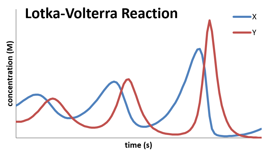
This mechanism follows kinetics predicted by what is called the predator-prey relationship. In this case, \(X\) represents the “prey” and \(Y\) represents the “predator”. The population of the predator cannot build up unless there is a significant population of prey on which the predators can feed. Likewise, the population of predators decreases when the population of the prey falls. And finally, there is a lag, as the rise and decline of the prey population controls the rise and fall of the predator population. The equations have been studied extensively and have applications not just in chemical kinetics, but in biology, economics, and elsewhere.

Steady-state approximation applied to Lotka-Volterra reaction¹

Species A being added to keep [A] constant implies that [A] = [A]_o, an unchanging constant.

The rate laws are:

\[\frac{d[X]}{dt} = k_1 [A]_o[X] - k_2[X][Y]\nonumber \]

\[\frac{d[Y]}{dt} =  k_2[X][Y] - k_3[Y]\nonumber \]

If [X] is in steady state:

\[0 =  k_1 [A]_o[X] - k_2[X][Y]  = [X]( k_1 [A]_o - k_2[Y])\nonumber \]

Which has two possible solutions: [X] = 0 or [Y] = k₁[A]_o/k₂. Applying the steady state to [Y] yields:

\[0 =  k_2[X][Y] - k_3[Y] = [Y]( k_2[X] - k_3) \implies [Y] = 0 \,\text{or}\, [X] = \frac{k_3}{k_2}\nonumber \]

So we now have two steady-state solutions for each species:

\[[X] = \frac{k_3}{k_2} \,\text{or}\, [X] = 0 \nonumber \]

\[[Y] = \frac{k_1[A]_o}{k_2} \,\text{or}\, [Y] = 0 \nonumber \]

This means that the reaction could oscillate between the two extremes for each species. Having multiple steady-state solutions for species is a hallmark of reactions that can oscillate. This is an example of an unstable (bistable) system. Reference 1 has a more detailed mathematical analysis of the time behavior where the oscillations are modeled as small excursions from the steady-state conditions   [Y]_ss = k₁[A]_o/k₂ and [X]_ss = k₃/k₂.

References

1. J. I. Steinfeld, J.S Francisco, W. L. Hase  Chemical Kinetics and Dynamics (Prentice-Hall, Inc, Englewood Cliffs, New Jersey, 1989) Sec. 5.3.

Contributors

• Patrick Fleming (CSU Eastbay)
• Jonathan Gutow (UW Oshkosh)