10.2: Entropy

Learning Objectives

• Predict the sign of the entropy changes in simple chemical reactions or processes. 
• Describe entropy in relation to the dispersal of energy in a system and connect this to the number of microstates. 

In thermochemistry (Chapter 5), we saw that energy is conserved according to the First Law of Thermodynamics. Changes in the internal energy (\(\Delta E\)) and the enthalpy (\(\Delta H\)) of a system describe the flow of energy between a system and its surroundings. However, these quantities alone do not determine whether a process is spontaneous.

For example, if a hot frying pan is placed in a sink of cold water, heat flows from the frying pan to the water until they reach the same temperature. This heat flow obeys the First Law of Thermodynamics: energy is conserved. The reverse process, the frying pan becoming hotter while the water cools further, never happens spontaneously, even though energy would still be conserved.

These examples show that we need a new thermodynamic quantity, entropy, to understand why processes are spontaneous.

Entropy (\(S\)) is a thermodynamic quantity that measures the dispersal of energy in a system. Chemical and physical changes in a system may be accompanied by either an increase or a decrease in the dispersal of energy in the system, corresponding to an increase in entropy (\(\Delta S > 0\)) or a decrease in entropy (\(\Delta S < 0\)), respectively. As with any other state function, the change in entropy is defined as the difference between the entropies of the final and initial states:

\[\Delta S = S_{final}-S_{initial} \nonumber\]

The units of \(\Delta S\) are J/(mol·K).

One way to calculate \(\Delta S\) for a reaction is to use tabulated values of the standard molar entropy (\(S^\circ\)), which is the entropy of 1 mol of a substance at a standard pressure of 1 atm and often reported at 298 K. Unlike enthalpy or internal energy, it is possible to obtain absolute entropy values by measuring the entropy change that occurs between the reference point of 0 K (corresponding to S = 0 J/(mol·K) for perfect crystalline substances) and the desired final temperature, typically 298 K.

Trends in Entropy

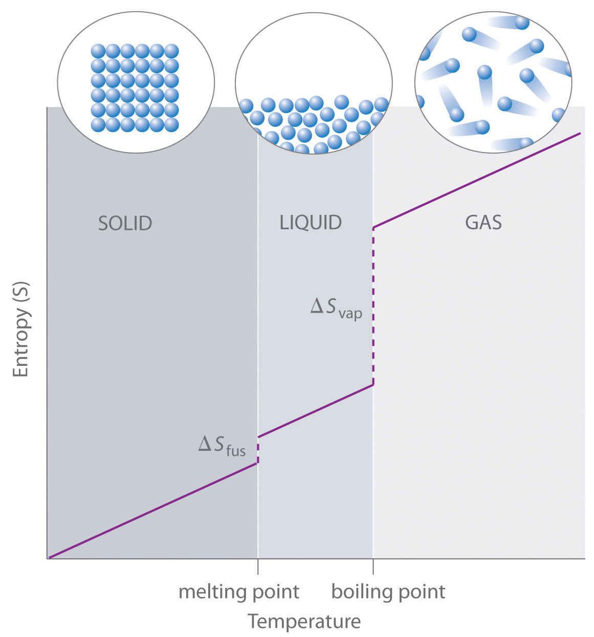
Consider the phase changes illustrated in Figure \(\PageIndex{1}\). In the solid phase, atoms or molecules are restricted to vibrating in nearly fixed positions. In the liquid phase, they are free to move over and around each other, though they remain in relatively close proximity. In the gas phase, the particles are much more widely dispersed and have much greater freedom of motion. Entropy increases because the number of possible arrangements of the particles and their motions increases with each phase change. For any substance: \[S_{solid}<S_{liquid}<<S_{gas}\nonumber\]

 

Figure \(\PageIndex{1}\): The entropy of a substance increases (ΔS > 0) as it transforms from a relatively ordered solid, to a less-ordered liquid, and then to a still less-ordered gas. Entropy decreases (ΔS < 0) as the substance transforms from a gas to a liquid and then to a solid.

The temperature of a substance is proportional to the average kinetic energy of its particles. As temperature increases (Figure \(\PageIndex{2}\)), molecules move more rapidly and can access a wider range of motions, including vibrations, rotations, and translations (Figure \(\PageIndex{3}\)). These motions become more extensive at higher temperatures, resulting in a greater dispersal of energy and an increase in entropy. Thus, the entropy for any substance increases with temperature.

Figure \(\PageIndex{2}\): Entropy versus Temperature. Entropy increases steadily with increasing temperature until the melting point is reached, where it jumps suddenly as the substance undergoes a phase change from a highly ordered solid to a disordered liquid (ΔS_fus). The entropy again increases steadily with increasing temperature until the boiling point is reached, where it jumps suddenly as the liquid undergoes a phase change to a highly disordered gas (ΔS_vap).

 

Figure \(\PageIndex{3}\): Molecular motions of a carbon dioxide molecule. Vibrational motion (left): the atoms within a molecule move relative to each other; Rotational motion (middle): the entire molecule rotates around any axis; Translational motion (right): the entire molecule moves in three dimensional space. These motions become more extensive at higher temperatures.

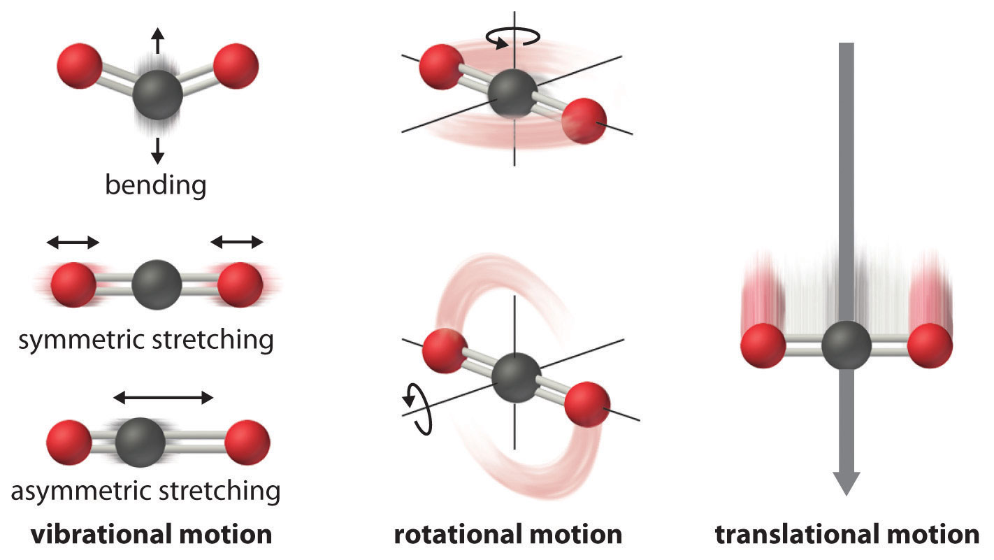
In addition, for substances in the same phase, entropy increases with molecular complexity, that is, with the number of atoms making up a molecule. The more atoms in the structure, the more molecular motions are possible. For example, carbon monoxide, (\(\ce{CO}\)) has only one vibrational motion possible with the carbon and oxygen atoms moving together and apart, compared to the three vibrational motions of carbon dioxide (\(\ce{CO2}\)) shown in Figure \(\PageIndex{3}\). Correspondingly, the standard molar entropy of \(\ce{CO2}\) is higher:

\[S^\circ(\ce{CO2})=213.8\; J/(mol⋅K) \: \text{vs} \: S^\circ(\ce{CO})=197.7\; J/(mol⋅K) \nonumber \]

Finally, variations in particle types affect the entropy of a system. Compared to a pure substance, a mixture of different types of particles has a greater entropy. This is due to the additional orientations and interactions possible among nonidentical components. For example, when a solid dissolves in a liquid, the particles of the solid experience greater freedom of motion and additional interactions with solvent particles. Dissolution typically results in an increase in entropy (\(\Delta S > 0\)).

Considering the various factors that affect entropy allows us to make informed predictions of the sign of \(\Delta S \) for various chemical and physical processes, as illustrated in Example \(\PageIndex{1}\).

Example \(\PageIndex{1}\): Predicting the Sign of ∆S

Predict the sign of the entropy change (\(\Delta S \)) for the following processes. Explain your prediction.

1. Heating one mole of liquid water from room temperature to 50 °C
2. \(\ce{Ag+ (aq) + Cl- (aq) \longrightarrow AgCl (s)}\)
3. \(\ce{C6H6(l) +\frac{15}{2} O2(g) \longrightarrow 6CO2(g) + 3 H2O(l)}\)
4. \(\ce{NH_3(s) \longrightarrow NH_3(l)}\)

Solution

1. Entropy increases (\(\Delta S > 0\)); temperature increases, leading to greater molecular motion.
2. Entropy decreases (\(\Delta S < 0\)); ions combine to form a solid, reducing dispersal of matter.
3. Entropy decreases (\(\Delta S < 0\)); net decrease in the number of gaseous molecules.
4. Entropy increases (\(\Delta S > 0\)); phase change from solid to liquid increases freedom of motion.

Exercise \(\PageIndex{1}\)

Predict the sign of the entropy change for the following processes. Give a reason for your prediction.

1. \(\ce{NaNO3 (s) \rightarrow Na+ (aq) + NO3- (aq) }\)
2. Freezing of liquid water
3. \(\ce{CO2 (s) \rightarrow CO2 (g)}\)
4. \(\ce{CaCO3 (s) \rightarrow CaO (s) + CO2 (g)}\)

Answer

a. Positive; the solid dissolves, increasing the number of mobile ions.

b. Negative; the liquid becomes a more ordered solid.

c. Positive; the ordered solid becomes a gas.

d. Positive; a gas forms

Microstates

Entropy corresponds to a larger dispersal of energy and more probable states. To understand why, we can examine entropy at the molecular scale. High-entropy states, which have greater energy dispersal and greater freedom of motion, can be achieved in more ways than low-entropy states. As a result, high-entropy states are more probable.

The entropy of a system can be related to the number of microstates (W) available to it. A microstate is a specific arrangement of all the positions and energies of the atoms or molecules that make up a system at a specific total energy. The relationship between a system’s entropy and the number of possible microstates is given by the Boltzmann equation:

\[S=k \ln W \nonumber \]

where k is the Boltzmann constant, 1.38 x 10⁻²³ J/K.

As for other state functions, the change in entropy for a process is the difference between its final and initial values:

\[\Delta S=S_{final}-S_{initial}=k \ln W_{final}-k \ln W_{initial}=k \ln \frac{W_{final}}{W_{initial}} \nonumber \]

If the number of microstates increases during a process (\(W_{final}>W_{initial}\)), the entropy of the system increases and \(\Delta S > 0\). If the number of microstates decreases during a process (\(W_{final}<W_{initial}\)), the entropy of the system decreases and \(\Delta S < 0\). This molecular-scale interpretation of entropy provides a link to the probability that a process will occur.

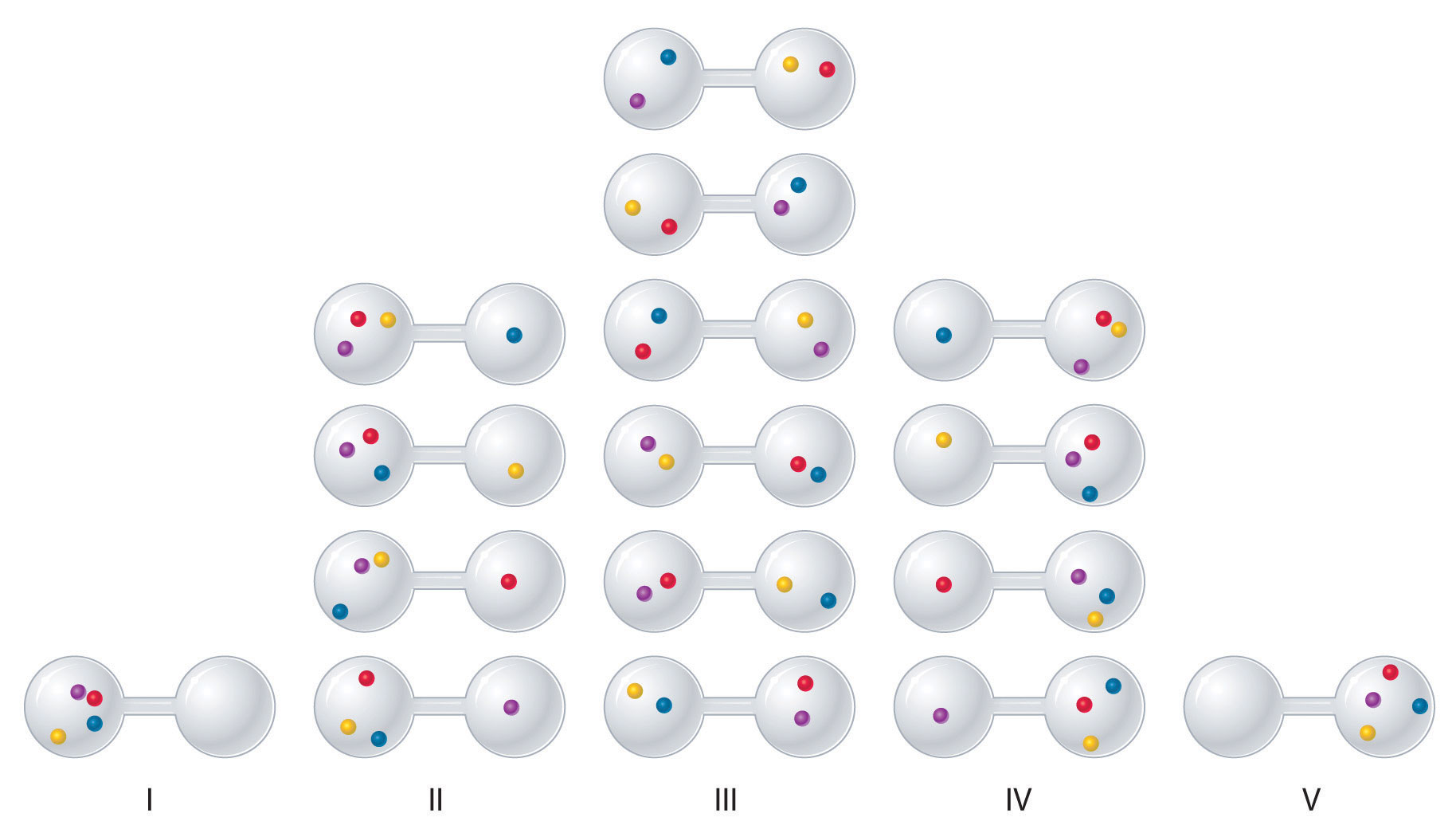
Suppose four gas molecules are initially confined to one side of a two-bulb container (Figure \(\PageIndex{4}\)). In this case, there is only one possible microstate: all four molecules must be in the same bulb.

When the valve between the bulbs is opened, the molecules are free to occupy either bulb. If we (artificially) distinguish the molecules by colour, we can see that there are 16 possible microstates overall. Some macroscopic arrangements (like all molecules in one bulb) correspond to just one microstate. Other arrangements (like two molecules in each bulb) correspond to multiple microstates.

• Arrangement I: 1 microstate
• Arrangement II: 4 microstates
• Arrangement III: 6 microstates
• Arrangement IV: 4 microstates
• Arrangement V: 1 microstate

Because the number of microstates increases when the molecules have more available space, the entropy of the system also increases.
Expansion increases entropy by increasing the number of accessible microstates.

Quantitatively, initially, there was one available microstate, W_initial = 1. Thus:

\[S_{initial} = k\ln(1)=(1.38 \times 10^{−23} J/K)(0) = 0 \nonumber\]

Here, S_initial = 0 means that in this simplified model, there is only one possible arrangement of molecules. It does not mean the gas actually has zero entropy; in reality, molecules have many other microstates from translational, rotational, vibrational, and electronic motion.

After the valve is opened, each of the four molecules (\(N=4\)) can be in either bulb (2 possible locations), leading to 16 microstates:

\[W_{final} = 2^N = 2^4 = 16\nonumber\]

\[S_{final} = k\ln W =(1.38 \times 10^{-23}J/K)\ln(16) = 3.83 \times 10^{-23} J/K \nonumber\]

This calculation confirms the conceptual idea: when the available volume increases, the number of positional microstates increases, and so does the entropy.

Note: This example focuses on the changes in microstates relating to the changes in the positions of the molecules in the two bulbs. Real gases have many more microstates, even before expansion, so their entropy is always greater than zero.

Figure \(\PageIndex{4}\): Distribution of four gas molecules between two connected containers.

Now imagine a real gas sample with 2.69 × 10²² molecules in a 1.00 L container. If this gas is allowed to expand into a second connected 1.00 L container, the number of positions available to each molecule doubles. The number of possible microstates is proportional to the volume and number of particles that make up the system:

\[W \propto V^N \nonumber\]

Increasing the volume by a factor of 2 results in an increase of the number of possible microstates by 2. The change in entropy upon changing the volume is:
\[\begin{aligned}
\Delta S&=S_{final}-S_{initial}=k \ln W_{final}-k \ln W_{initial} =k \ln \frac{W_{final}}{W_{initial}} = k\ln \left( \frac{V_{final}}{V_{initial}} \right)^N\\ &=1.38 \times 10^{−23} J/K\ln \left(\frac{2.00 L}{1.00 L} \right)^{2.69 \times 10^{22}}=1.38 \times 10^{−23} J/K(2.69 \times 10^{22})\ln2 =0.257 J/K \end{aligned}\nonumber \]

This simple calculation shows that increasing the number of available microstates leads to an increase in entropy.

Although we will not use Boltzmann’s equation for entropy calculations in CHM 135, reviewing these calculations helps develop a conceptual understanding of the relationship between microstates, probability, and entropy.

Let's look back at phase changes in terms of microstates:

• Solid to liquid (melting):
  In a solid, atoms or molecules occupy fixed positions in a lattice. In a liquid, particles are free to move and tumble, allowing many more microstates.
  ΔS_fus > 0
   
• Liquid to gas (vaporization):
  Molecules in a gas have even greater freedom of motion than in a liquid, so
  ΔS_vap > 0

Conversely, the reverse processes, condensation and freezing, reduce freedom of motion and the number of microstates, and thus decrease entropy.

Each increase in freedom of motion corresponds to an increase in the number of accessible microstates, making higher-entropy states both more probable and more stable.

Example \(\PageIndex{2}\): Comparing Entropies based on Microstates

Predict which substance in each pair has the higher entropy and justify your answer.

1. 1 mol of NH₃(g) or 1 mol of He(g), both at 25°C
2. 1 mol of Pb(s) at 25°C or 1 mol of Pb(l) at 800°C

Given: amounts of substances and temperature

Asked for: higher entropy

Strategy:

From the number of atoms present and the phase of each substance, predict which has the greater number of available microstates and hence the higher entropy.

Solution:

1. Both substances are gases at 25°C, but one consists of He atoms and the other consists of NH₃ molecules. With four atoms instead of one, the NH₃ molecules have more motions available, leading to a greater number of microstates. Hence we predict that the NH₃ sample will have the higher entropy.
2. The nature of the atomic species is the same in both cases, but the phase is different: one sample is a solid, and one is a liquid. Based on the greater freedom of motion available to atoms in a liquid (more microstates), we predict that the liquid sample will have the higher entropy.

Summary

Entropy (\(S\)) is a state function that measures the dispersal of energy in a system and is related to the number of accessible microstates. A greater number of microstates corresponds to a more probable state and a higher entropy.

Entropy increases with temperature, phase changes (solid → liquid → gas), molecular complexity, and mixing.