
13.2: Equilibrium Constants
- Page ID
- 105633

\( \newcommand{\vecs}[1]{\overset { \scriptstyle \rightharpoonup} {\mathbf{#1}} } \)
\( \newcommand{\vecd}[1]{\overset{-\!-\!\rightharpoonup}{\vphantom{a}\smash {#1}}} \)
\( \newcommand{\dsum}{\displaystyle\sum\limits} \)
\( \newcommand{\dint}{\displaystyle\int\limits} \)
\( \newcommand{\dlim}{\displaystyle\lim\limits} \)
\( \newcommand{\id}{\mathrm{id}}\) \( \newcommand{\Span}{\mathrm{span}}\)
( \newcommand{\kernel}{\mathrm{null}\,}\) \( \newcommand{\range}{\mathrm{range}\,}\)
\( \newcommand{\RealPart}{\mathrm{Re}}\) \( \newcommand{\ImaginaryPart}{\mathrm{Im}}\)
\( \newcommand{\Argument}{\mathrm{Arg}}\) \( \newcommand{\norm}[1]{\| #1 \|}\)
\( \newcommand{\inner}[2]{\langle #1, #2 \rangle}\)
\( \newcommand{\Span}{\mathrm{span}}\)
\( \newcommand{\id}{\mathrm{id}}\)
\( \newcommand{\Span}{\mathrm{span}}\)
\( \newcommand{\kernel}{\mathrm{null}\,}\)
\( \newcommand{\range}{\mathrm{range}\,}\)
\( \newcommand{\RealPart}{\mathrm{Re}}\)
\( \newcommand{\ImaginaryPart}{\mathrm{Im}}\)
\( \newcommand{\Argument}{\mathrm{Arg}}\)
\( \newcommand{\norm}[1]{\| #1 \|}\)
\( \newcommand{\inner}[2]{\langle #1, #2 \rangle}\)
\( \newcommand{\Span}{\mathrm{span}}\) \( \newcommand{\AA}{\unicode[.8,0]{x212B}}\)
\( \newcommand{\vectorA}[1]{\vec{#1}} % arrow\)
\( \newcommand{\vectorAt}[1]{\vec{\text{#1}}} % arrow\)
\( \newcommand{\vectorB}[1]{\overset { \scriptstyle \rightharpoonup} {\mathbf{#1}} } \)
\( \newcommand{\vectorC}[1]{\textbf{#1}} \)
\( \newcommand{\vectorD}[1]{\overrightarrow{#1}} \)
\( \newcommand{\vectorDt}[1]{\overrightarrow{\text{#1}}} \)
\( \newcommand{\vectE}[1]{\overset{-\!-\!\rightharpoonup}{\vphantom{a}\smash{\mathbf {#1}}}} \)
\( \newcommand{\vecs}[1]{\overset { \scriptstyle \rightharpoonup} {\mathbf{#1}} } \)
\(\newcommand{\longvect}{\overrightarrow}\)
\( \newcommand{\vecd}[1]{\overset{-\!-\!\rightharpoonup}{\vphantom{a}\smash {#1}}} \)
\(\newcommand{\avec}{\mathbf a}\) \(\newcommand{\bvec}{\mathbf b}\) \(\newcommand{\cvec}{\mathbf c}\) \(\newcommand{\dvec}{\mathbf d}\) \(\newcommand{\dtil}{\widetilde{\mathbf d}}\) \(\newcommand{\evec}{\mathbf e}\) \(\newcommand{\fvec}{\mathbf f}\) \(\newcommand{\nvec}{\mathbf n}\) \(\newcommand{\pvec}{\mathbf p}\) \(\newcommand{\qvec}{\mathbf q}\) \(\newcommand{\svec}{\mathbf s}\) \(\newcommand{\tvec}{\mathbf t}\) \(\newcommand{\uvec}{\mathbf u}\) \(\newcommand{\vvec}{\mathbf v}\) \(\newcommand{\wvec}{\mathbf w}\) \(\newcommand{\xvec}{\mathbf x}\) \(\newcommand{\yvec}{\mathbf y}\) \(\newcommand{\zvec}{\mathbf z}\) \(\newcommand{\rvec}{\mathbf r}\) \(\newcommand{\mvec}{\mathbf m}\) \(\newcommand{\zerovec}{\mathbf 0}\) \(\newcommand{\onevec}{\mathbf 1}\) \(\newcommand{\real}{\mathbb R}\) \(\newcommand{\twovec}[2]{\left[\begin{array}{r}#1 \\ #2 \end{array}\right]}\) \(\newcommand{\ctwovec}[2]{\left[\begin{array}{c}#1 \\ #2 \end{array}\right]}\) \(\newcommand{\threevec}[3]{\left[\begin{array}{r}#1 \\ #2 \\ #3 \end{array}\right]}\) \(\newcommand{\cthreevec}[3]{\left[\begin{array}{c}#1 \\ #2 \\ #3 \end{array}\right]}\) \(\newcommand{\fourvec}[4]{\left[\begin{array}{r}#1 \\ #2 \\ #3 \\ #4 \end{array}\right]}\) \(\newcommand{\cfourvec}[4]{\left[\begin{array}{c}#1 \\ #2 \\ #3 \\ #4 \end{array}\right]}\) \(\newcommand{\fivevec}[5]{\left[\begin{array}{r}#1 \\ #2 \\ #3 \\ #4 \\ #5 \\ \end{array}\right]}\) \(\newcommand{\cfivevec}[5]{\left[\begin{array}{c}#1 \\ #2 \\ #3 \\ #4 \\ #5 \\ \end{array}\right]}\) \(\newcommand{\mattwo}[4]{\left[\begin{array}{rr}#1 \amp #2 \\ #3 \amp #4 \\ \end{array}\right]}\) \(\newcommand{\laspan}[1]{\text{Span}\{#1\}}\) \(\newcommand{\bcal}{\cal B}\) \(\newcommand{\ccal}{\cal C}\) \(\newcommand{\scal}{\cal S}\) \(\newcommand{\wcal}{\cal W}\) \(\newcommand{\ecal}{\cal E}\) \(\newcommand{\coords}[2]{\left\{#1\right\}_{#2}}\) \(\newcommand{\gray}[1]{\color{gray}{#1}}\) \(\newcommand{\lgray}[1]{\color{lightgray}{#1}}\) \(\newcommand{\rank}{\operatorname{rank}}\) \(\newcommand{\row}{\text{Row}}\) \(\newcommand{\col}{\text{Col}}\) \(\renewcommand{\row}{\text{Row}}\) \(\newcommand{\nul}{\text{Nul}}\) \(\newcommand{\var}{\text{Var}}\) \(\newcommand{\corr}{\text{corr}}\) \(\newcommand{\len}[1]{\left|#1\right|}\) \(\newcommand{\bbar}{\overline{\bvec}}\) \(\newcommand{\bhat}{\widehat{\bvec}}\) \(\newcommand{\bperp}{\bvec^\perp}\) \(\newcommand{\xhat}{\widehat{\xvec}}\) \(\newcommand{\vhat}{\widehat{\vvec}}\) \(\newcommand{\uhat}{\widehat{\uvec}}\) \(\newcommand{\what}{\widehat{\wvec}}\) \(\newcommand{\Sighat}{\widehat{\Sigma}}\) \(\newcommand{\lt}{<}\) \(\newcommand{\gt}{>}\) \(\newcommand{\amp}{&}\) \(\definecolor{fillinmathshade}{gray}{0.9}\)Skills to Develop
- Derive reaction quotients from chemical equations representing homogeneous and heterogeneous reactions
- Calculate values of reaction quotients and equilibrium constants, using concentrations and pressures
- Relate the magnitude of an equilibrium constant to properties of the chemical system
Now that we have a symbol (\(\rightleftharpoons\)) to designate reversible reactions, we will need a way to express mathematically how the amounts of reactants and products affect the equilibrium of the system. A general equation for a reversible reaction may be written as follows:
\[m\ce{A}+n\ce{B}+ \rightleftharpoons x\ce{C}+y\ce{D} \label{13.3.1}\]
We can write the reaction quotient (\(Q\)) for this equation. When evaluated using concentrations, it is called \(Q_c\). We use brackets to indicate molar concentrations of reactants and products.
\[ Q_c=\dfrac{[\ce{C}]^x[\ce{D}]^y}{[\ce{A}]^m[\ce{B}]^n} \label{13.3.2}\]
The reaction quotient is equal to the molar concentrations of the products of the chemical equation (multiplied together) over the reactants (also multiplied together), with each concentration raised to the power of the coefficient of that substance in the balanced chemical equation. For example, the reaction quotient for the reversible reaction
\[\ce{2NO}_{2(g)} \rightleftharpoons \ce{N_2O}_{4(g)} \label{13.3.3}\]
is given by this expression:
\[Q_c=\ce{\dfrac{[N_2O_4]}{[NO_2]^2}} \label{13.3.4}\]
Example \(\PageIndex{1}\): Writing Reaction Quotient Expressions
Write the expression for the reaction quotient for each of the following reactions:
- \(\ce{3O}_{2(g)} \rightleftharpoons \ce{2O}_{3(g)}\)
- \(\ce{N}_{2(g)}+\ce{3H}_{2(g)} \rightleftharpoons \ce{2NH}_{3(g)}\)
- \(\ce{4NH}_{3(g)}+\ce{7O}_{2(g)} \rightleftharpoons \ce{4NO}_{2(g)}+\ce{6H_2O}_{(g)}\)
Solution
- \(Q_c=\dfrac{[\ce{O3}]^2}{[\ce{O2}]^3}\)
- \( Q_c=\dfrac{[\ce{NH3}]^2}{\ce{[N2][H2]}^3}\)
- \( Q_c=\dfrac{\ce{[NO2]^4[H2O]^6}}{\ce{[NH3]^4[O2]^7}}\)
Exercise \(\PageIndex{1}\)
Write the expression for the reaction quotient for each of the following reactions:
- \( \ce{2SO2}(g)+\ce{O2}(g) \rightleftharpoons \ce{2SO3}(g)\)
- \( \ce{C4H8}(g) \rightleftharpoons \ce{2C2H4}(g)\)
- \( \ce{2C4H10}(g)+\ce{13O2}(g) \rightleftharpoons \ce{8CO2}(g)+\ce{10H2O}(g)\)
- Answer a
-
\( Q_c=\dfrac{[\ce{SO3}]^2}{\ce{[SO2]^2[O2]}}\)
- Answer b
-
\( Q_c=\dfrac{[\ce{C2H4}]^2}{[\ce{C4H8}]}\)
- Answer c
-
\( Q_c=\dfrac{\ce{[CO2]^8[H2O]^{10}}}{\ce{[C4H10]^2[O2]^{13}}}\)
The numeric value of \(Q_c\) for a given reaction varies; it depends on the concentrations of products and reactants present at the time when \(Q_c\) is determined. When pure reactants are mixed, \(Q_c\) is initially zero because there are no products present at that point. As the reaction proceeds, the value of \(Q_c\) increases as the concentrations of the products increase and the concentrations of the reactants simultaneously decrease (Figure \(\PageIndex{1}\)). When the reaction reaches equilibrium, the value of the reaction quotient no longer changes because the concentrations no longer change.
![Three graphs are shown and labeled, “a,” “b,” and “c.” All three graphs have a vertical dotted line running through the middle labeled, “Equilibrium is reached.” The y-axis on graph a is labeled, “Concentration,” and the x-axis is labeled, “Time.” Three curves are plotted on graph a. The first is labeled, “[ S O subscript 2 ];” this line starts high on the y-axis, ends midway down the y-axis, has a steep initial slope and a more gradual slope as it approaches the far right on the x-axis. The second curve on this graph is labeled, “[ O subscript 2 ];” this line mimics the first except that it starts and ends about fifty percent lower on the y-axis. The third curve is the inverse of the first in shape and is labeled, “[ S O subscript 3 ].” The y-axis on graph b is labeled, “Concentration,” and the x-axis is labeled, “Time.” Three curves are plotted on graph b. The first is labeled, “[ S O subscript 2 ];” this line starts low on the y-axis, ends midway up the y-axis, has a steep initial slope and a more gradual slope as it approaches the far right on the x-axis. The second curve on this graph is labeled, “[ O subscript 2 ];” this line mimics the first except that it ends about fifty percent lower on the y-axis. The third curve is the inverse of the first in shape and is labeled, “[ S O subscript 3 ].” The y-axis on graph c is labeled, “Reaction Quotient,” and the x-axis is labeled, “Time.” A single curve is plotted on graph c. This curve begins at the bottom of the y-axis and rises steeply up near the top of the y-axis, then levels off into a horizontal line. The top point of this line is labeled, “k.”](https://chem.libretexts.org/@api/deki/files/137802/CNX_Chem_13_02_quotient.jpg?revision=1&size=bestfit&width=660)
Figure \(\PageIndex{1}\): (a) The change in the concentrations of reactants and products is depicted as the \(\ce{2SO2}(g)+\ce{O2}(g) \rightleftharpoons \ce{2SO3}(g)\) reaction approaches equilibrium. (b) The change in concentrations of reactants and products is depicted as the reaction \(\ce{2SO3}(g) \rightleftharpoons \ce{2SO2}(g)+\ce{O2}(g)\) approaches equilibrium. (c) The graph shows the change in the value of the reaction quotient as the reaction approaches equilibrium.
When a mixture of reactants and products of a reaction reaches equilibrium at a given temperature, its reaction quotient always has the same value. This value is called the equilibrium constant (\(K\)) of the reaction at that temperature. As for the reaction quotient, when evaluated in terms of concentrations, it is noted as \(K_c\).
That a reaction quotient always assumes the same value at equilibrium can be expressed as:
\[Q_c \textrm{ at equilibrium}=K_c=\dfrac{[\ce C]^x[\ce D]^y...}{[\ce A]^m[\ce B]^n...} \label{13.3.5}\]
This equation is a mathematical statement of the law of mass action: When a reaction has attained equilibrium at a given temperature, the reaction quotient for the reaction always has the same value.
Example \(\PageIndex{2}\): Evaluating a Reaction Quotient
Gaseous nitrogen dioxide forms dinitrogen tetroxide according to this equation:
\[\ce{2NO}_{2(g)} \rightleftharpoons \ce{N_2O}_{4(g)} \nonumber \]
When 0.10 mol \(\ce{NO2}\) is added to a 1.0-L flask at 25 °C, the concentration changes so that at equilibrium, [NO2] = 0.016 M and [N2O4] = 0.042 M.
- What is the value of the reaction quotient before any reaction occurs?
- What is the value of the equilibrium constant for the reaction?
Solution
- Before any product is formed, \(\mathrm{[NO_2]=\dfrac{0.10\:mol}{1.0\:L}}=0.10\:M\), and [N2O4] = 0 M. Thus, \[Q_c=\ce{\dfrac{[N2O4]}{[NO2]^2}}=\dfrac{0}{0.10^2}=0\]
- At equilibrium, the value of the equilibrium constant is equal to the value of the reaction quotient. At equilibrium, \[K_c=Q_c=\ce{\dfrac{[N2O4]}{[NO2]^2}}=\dfrac{0.042}{0.016^2}=1.6\times 10^2.\]
The equilibrium constant is 1.6 × 10².
Note that dimensional analysis would suggest the unit for this \(K_c\) value should be M−1. However, it is common practice to omit units for \(K_c\) values computed as described here, since it is the magnitude of an equilibrium constant that relays useful information. As will be discussed later in this module, the rigorous approach to computing equilibrium constants uses dimensionless quantities derived from concentrations instead of actual concentrations, and so \(K_c\) values are truly unitless.
Exercise \(\PageIndex{2}\)
For the reaction
\[\ce{2SO2}(g)+\ce{O2}(g) \rightleftharpoons \ce{2SO3}(g) \nonumber \]
the concentrations at equilibrium are [SO2] = 0.90 M, [O2] = 0.35 M, and [SO3] = 1.1 M. What is the value of the equilibrium constant, Kc?
- Answer
-
Kc = 4.3
The magnitude of an equilibrium constant is a measure of the yield of a reaction when it reaches equilibrium. A large value for \(K_c\) indicates that equilibrium is attained only after the reactants have been largely converted into products. A small value of \(K_c\)—much less than 1—indicates that equilibrium is attained when only a small proportion of the reactants have been converted into products.
Once a value of \(K_c\) is known for a reaction, it can be used to predict directional shifts when compared to the value of \(Q_c\). A system that is not at equilibrium will proceed in the direction that establishes equilibrium. The data in Figure \(\PageIndex{2}\) illustrate this. When heated to a consistent temperature, 800 °C, different starting mixtures of \(\ce{CO}\), \(\ce{H_2O}\), \(\ce{CO_2}\), and \(\ce{H_2}\) react to reach compositions adhering to the same equilibrium (the value of \(Q_c\) changes until it equals the value of Kc). This value is 0.640, the equilibrium constant for the reaction under these conditions.
\[\ce{CO}(g)+\ce{H2O}(g) \rightleftharpoons \ce{CO2}(g)+\ce{H2}(g) \hspace{20px} K_c=0.640 \hspace{20px} \mathrm{T=800°C} \label{13.3.6}\]
It is important to recognize that an equilibrium can be established starting either from reactants or from products, or from a mixture of both. For example, equilibrium was established from Mixture 2 in Figure \(\PageIndex{2}\) when the products of the reaction were heated in a closed container. In fact, one technique used to determine whether a reaction is truly at equilibrium is to approach equilibrium starting with reactants in one experiment and starting with products in another. If the same value of the reaction quotient is observed when the concentrations stop changing in both experiments, then we may be certain that the system has reached equilibrium.
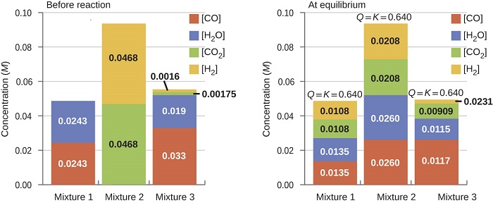
Figure \(\PageIndex{2}\): Concentrations of three mixtures are shown before and after reaching equilibrium at 800 °C for the so-called water gas shift reaction (Equation \ref{13.3.6}).
Example \(\PageIndex{3}\): Predicting the Direction of Reaction
Given here are the starting concentrations of reactants and products for three experiments involving this reaction:
\[\ce{CO}(g)+\ce{H2O}(g) \rightleftharpoons \ce{CO2}(g)+\ce{H2}(g) \nonumber\]
with \(K_c=0.64 \). Determine in which direction the reaction proceeds as it goes to equilibrium in each of the three experiments shown.
| Reactants/Products | Experiment 1 | Experiment 2 | Experiment 3 |
|---|---|---|---|
| [CO]i | 0.0203 M | 0.011 M | 0.0094 M |
| [H2O]i | 0.0203 M | 0.0011 M | 0.0025 M |
| [CO2]i | 0.0040 M | 0.037 M | 0.0015 M |
| [H2]i | 0.0040 M | 0.046 M | 0.0076 M |
Solution
Experiment 1:
Qc < \(K_c\) (0.039 < 0.64)
The reaction will shift to the right.
Experiment 2:
\[Q_c=\ce{\dfrac{[CO2][H2]}{[CO][H2O]}}=\dfrac{(0.037)(0.046)}{(0.011)(0.0011)}=1.4 \times 10^2 \nonumber\]
Qc > \(K_c\) (140 > 0.64)
The reaction will shift to the left.
Experiment 3:
Qc < \(K_c\) (0.48 < 0.64)
The reaction will shift to the right.
Exercise \(\PageIndex{3}\)
Calculate the reaction quotient and determine the direction in which each of the following reactions will proceed to reach equilibrium.
(a) A 1.00-L flask containing 0.0500 mol of NO(g), 0.0155 mol of Cl2(g), and 0.500 mol of NOCl:
\[\ce{2NO}(g)+\ce{Cl2}(g)⇌\ce{2NOCl}(g)\hspace{20px}K_c=4.6\times 10^4 \nonumber\]
(b) A 5.0-L flask containing 17 g of NH3, 14 g of N2, and 12 g of H2:
\[\ce{N2}(g)+\ce{3H2}(g)⇌\ce{2NH3}(g)\hspace{20px}K_c=0.060 \nonumber\]
(c) A 2.00-L flask containing 230 g of SO3(g):
\[\ce{2SO3}(g)⇌\ce{2SO2}(g)+\ce{O2}(g)\hspace{20px}K_c=0.230 \nonumber\]
- Answer a
-
\(Q_c\) = 6.45 × 10³, shifts right.
- Answer b
-
\(Q_c\) = 0.12, shifts left.
- Answer c
-
\(Q_c\) = 0, shifts right
In Example \(\PageIndex{2}\), it was mentioned that the common practice is to omit units when evaluating reaction quotients and equilibrium constants. It should be pointed out that using concentrations in these computations is a convenient but simplified approach that sometimes leads to results that seemingly conflict with the law of mass action. For example, equilibria involving aqueous ions often exhibit equilibrium constants that vary quite significantly (are not constant) at high solution concentrations. This may be avoided by computing \(K_c\) values using the activities of the reactants and products in the equilibrium system instead of their concentrations. The activity of a substance is a measure of its effective concentration under specified conditions. While a detailed discussion of this important quantity is beyond the scope of an introductory text, it is necessary to be aware of a few important aspects:
- Activities are dimensionless (unitless) quantities and are in essence “adjusted” concentrations.
- For relatively dilute solutions, a substance's activity and its molar concentration are roughly equal.
- Activities for pure condensed phases (solids and liquids) are equal to 1.
As a consequence of this last consideration, \(Q_c\) and \(K_c\) expressions do not contain terms for solids or liquids (being numerically equal to 1, these terms have no effect on the expression's value). Several examples of equilibria yielding such expressions will be encountered in this section.
Homogeneous Equilibria
A homogeneous equilibrium is one in which all of the reactants and products are present in a single solution (by definition, a homogeneous mixture). In this chapter, we will concentrate on the two most common types of homogeneous equilibria: those occurring in liquid-phase solutions and those involving exclusively gaseous species. Reactions between solutes in liquid solutions belong to one type of homogeneous equilibria. The chemical species involved can be molecules, ions, or a mixture of both. Several examples are provided here:
Example 1
\[\ce{C2H2}(aq)+\ce{2Br2}(aq) \rightleftharpoons \ce{C2H2Br4}(aq)\hspace{20px} \label{13.3.7a}\]
with associated equilibrium constant
\[K_c=\ce{\dfrac{[C2H2Br4]}{[C2H2][Br2]^2}} \label{13.3.7b}\]
Example 2
\[\ce{I2}(aq)+\ce{I-}(aq) \rightleftharpoons \ce{I3-}(aq) \label{13.3.8b}\]
with associated equilibrium constant
\[K_c=\ce{\dfrac{[I3- ]}{[I2][I- ]}} \label{13.3.8c}\]
Example 3
\[\ce{Hg2^2+}(aq)+\ce{NO3-}(aq)+\ce{3H3O+}(aq) \rightleftharpoons \ce{2Hg^2+}(aq)+\ce{HNO2}(aq)+\ce{4H2O}(l) \label{13.3.9a}\]
with associated equilibrium constant
\[K_c=\ce{\dfrac{[Hg^2+]^2[HNO2]}{[Hg2^2+][NO3- ][H3O+]^3}} \label{13.3.9b}\]
Example 4
\[\ce{HF}(aq)+\ce{H2O}(l) \rightleftharpoons \ce{H3O+}(aq)+\ce{F-}(aq) \label{13.3.10a}\]
with associated equilibrium constant
\[K_c=\ce{\dfrac{[H3O+][F- ]}{[HF]}} \label{13.3.10b}\]
Example 5
\[\ce{NH3}(aq)+\ce{H2O}(l) \rightleftharpoons \ce{NH4+}(aq)+\ce{OH-}(aq) \label{13.3.11a}\]
with associated equilibrium constant
\[K_c=\ce{\dfrac{[NH4+][OH- ]}{[NH3]}} \label{13.3.11b}\]
In each of these examples, the equilibrium system is an aqueous solution, as denoted by the aq annotations on the solute formulas. Since H2O(l) is the solvent for these solutions, its concentration does not appear as a term in the \(K_c\) expression, as discussed earlier, even though it may also appear as a reactant or product in the chemical equation.
Reactions in which all reactants and products are gases represent a second class of homogeneous equilibria. We use molar concentrations in the following examples, but we will see shortly that partial pressures of the gases may be used as well:
Example 1
\[\ce{C2H6}(g) \rightleftharpoons \ce{C2H4}(g)+\ce{H2}(g) \label{13.3.12a}\]
with associated equilibrium constant
\[K_c=\ce{\dfrac{[C2H4][H2]}{[C2H6]}} \label{13.3.12b}\]
Example 2
\[\ce{3O2}(g) \rightleftharpoons \ce{2O3}(g) \label{13.3.13a}\]
with associated equilibrium constant
\[K_c=\ce{\dfrac{[O3]^2}{[O2]^3}} \label{13.3.13b}\]
Example 3
\[\ce{N2}(g)+\ce{3H2}(g) \rightleftharpoons \ce{2NH3}(g) \label{13.3.14a}\]
with associated equilibrium constant
\[K_c=\ce{\dfrac{[NH3]^2}{[N2][H2]^3}} \label{13.3.14b}\]
Example 4
\[\ce{C3H8}(g)+\ce{5O2}(g) \rightleftharpoons \ce{3CO2}(g)+\ce{4H2O}(g)\label{13.3.15a} \]
with associated equilibrium constant
\[K_c=\ce{\dfrac{[CO2]^3[H2O]^4}{[C3H8][O2]^5}}\label{13.3.15b}\]
Note that the concentration of \(\ce{H_2O}_{(g)}\) has been included in the last example because water is not the solvent in this gas-phase reaction and its concentration (and activity) changes.
Whenever gases are involved in a reaction, the partial pressure of each gas can be used instead of its concentration in the equation for the reaction quotient because the partial pressure of a gas is directly proportional to its concentration at constant temperature. This relationship can be derived from the ideal gas equation, where M is the molar concentration of gas, \(\dfrac{n}{V}\).
\[PV=nRT \label{13.3.16}\]
\[P=\left(\dfrac{n}{V}\right)RT \label{13.3.17}\]
\[=MRT \label{13.3.18}\]
Thus, at constant temperature, the pressure of a gas is directly proportional to its concentration. Using the partial pressures of the gases, we can write the reaction quotient for the system
\[\ce{C2H6}(g) \rightleftharpoons \ce{C2H4}(g)+\ce{H2}(g) \label{13.3.19}\]
by following the same guidelines for deriving concentration-based expressions:
\[Q_P=\dfrac{P_{\ce{C2H4}}P_{\ce{H2}}}{P_{\ce{C2H6}}} \label{13.3.20}\]
In this equation we use QP to indicate a reaction quotient written with partial pressures: \(P_{\ce{C2H6}}\) is the partial pressure of C2H6; \(P_{\ce{H2}}\), the partial pressure of H2; and \(P_{\ce{C2H6}}\), the partial pressure of C2H4. At equilibrium:
\[K_P=Q_P=\dfrac{P_{\ce{C2H4}}P_{\ce{H2}}}{P_{\ce{C2H6}}} \label{13.3.21}\]
The subscript \(P\) in the symbol \(K_P\) designates an equilibrium constant derived using partial pressures instead of concentrations. The equilibrium constant, KP, is still a constant, but its numeric value may differ from the equilibrium constant found for the same reaction by using concentrations.
Conversion between a value for \(K_c\), an equilibrium constant expressed in terms of concentrations, and a value for \(K_P\), an equilibrium constant expressed in terms of pressures, is straightforward (a K or Q without a subscript could be either concentration or pressure).
The equation relating \(K_c\) and \(K_P\) is derived as follows. For the gas-phase reaction:
\[m\ce{A}+n\ce{B} \rightleftharpoons x\ce{C}+y\ce{D} \label{13.3.22}\]
with
\[K_P=\dfrac{(P_C)^x(P_D)^y}{(P_A)^m(P_B)^n} \label{13.3.23}\]
\[=\dfrac{([\ce C]×RT)^x([\ce D]×RT)^y}{([\ce A]×RT)^m([\ce B]×RT)^n} \label{13.3.24}\]
\[=\dfrac{[\ce C]^x[\ce D]^y}{[\ce A]^m[\ce B]^n}×\dfrac{(RT)^{x+y}}{(RT)^{m+n}} \label{13.3.25}\]
\[=K_c(RT)^{(x+y)−(m+n)} \label{13.3.26}\]
\[=K_c(RT)^{Δn} \label{13.3.27}\]
The relationship between \(K_c\) and \(K_P\) is
In this equation, Δn is the difference between the sum of the coefficients of the gaseous products and the sum of the coefficients of the gaseous reactants in the reaction (the change in moles of gas between the reactants and the products). For the gas-phase reaction \(m\ce{A}+n\ce{B} \rightleftharpoons x\ce{C}+y\ce{D}\), we have
Example \(\PageIndex{4}\): Calculation of KP
Write the equations for the conversion of \(K_c\) to KP for each of the following reactions:
- \(\ce{C2H6}(g) \rightleftharpoons \ce{C2H4}(g)+\ce{H2}(g)\)
- \(\ce{CO}(g)+\ce{H2O}(g) \rightleftharpoons \ce{CO2}(g)+\ce{H2}(g)\)
- \(\ce{N2}(g)+\ce{3H2}(g) \rightleftharpoons \ce{2NH3}(g)\)
- Kc is equal to 0.28 for the following reaction at 900 °C:
\[\ce{CS2}(g)+\ce{4H2}(g) \rightleftharpoons \ce{CH4}(g)+\ce{2H2S}(g)\]
What is KP at this temperature?
Solution
(a) Δn = (2) − (1) = 1
KP = \(K_c\) (RT)Δn = \(K_c\) (RT)1 = \(K_c\) (RT)
(b) Δn = (2) − (2) = 0
KP = \(K_c\) (RT)Δn = \(K_c\) (RT)0 = Kc
(c) Δn = (2) − (1 + 3) = −2
KP = \(K_c\) (RT)Δn = \(K_c\) (RT)−2 = \(\dfrac{K_c}{(RT)^2}\)
d) KP = \(K_c\) (RT)Δn = (0.28)[(0.0821)(1173)]−2 = 3.0 × 10⁻⁵
Exercise \(\PageIndex{4}\)
Write the equations for the conversion of \(K_c\) to KP for each of the following reactions, which occur in the gas phase:
- \(\ce{2SO2}(g)+\ce{O2}(g) \rightleftharpoons \ce{2SO3}(g)\)
- \(\ce{N2O4}(g) \rightleftharpoons \ce{2NO2}(g)\)
- \(\ce{C3H8}(g)+\ce{5O2}(g) \rightleftharpoons \ce{3CO2}(g)+\ce{4H2O}(g)\)
- At 227 °C, the following reaction has \(K_c\) = 0.0952:
\[\ce{CH3OH}(g) \rightleftharpoons \ce{CO}(g)+\ce{2H2}(g)\]
What would be the value of KP at this temperature?
- Answer a
-
KP = \(K_c\) (RT)−1
- Answer b
-
KP = \(K_c\) (RT)
- Answer c
-
KP = \(K_c\) (RT);
- Answer d
-
160 or 1.6 × 10²
Heterogeneous Equilibria
A heterogeneous equilibrium is a system in which reactants and products are found in two or more phases. The phases may be any combination of solid, liquid, or gas phases, and solutions. When dealing with these equilibria, remember that solids and pure liquids do not appear in equilibrium constant expressions (the activities of pure solids, pure liquids, and solvents are 1).
Some heterogeneous equilibria involve chemical changes:
Example 1
\[\ce{PbCl2}(s) \rightleftharpoons \ce{Pb^2+}(aq)+\ce{2Cl-}(aq) \label{13.3.30a}\]
with associated equilibrium constant
\[K_c=\ce{[Pb^2+][Cl- ]^2} \label{13.3.30b}\]
Example 1
\[\ce{CaO}(s)+\ce{CO2}(g) \rightleftharpoons \ce{CaCO3}(s) \label{13.3.31a}\]
with associated equilibrium constant
\[K_c=\dfrac{1}{[\ce{CO2}]} \label{13.3.31b}\]
Example 1
\[\ce{C}(s)+\ce{2S}(g) \rightleftharpoons \ce{CS2}(g) \label{13.3.32a}\]
with associated equilibrium constant
\[K_c=\ce{\dfrac{[CS2]}{[S]^2}} \label{13.3.32b}\]
Other heterogeneous equilibria involve phase changes, for example, the evaporation of liquid bromine, as shown in the following equation:
\[\ce{Br2}(l) \rightleftharpoons \ce{Br2}(g) \label{13.3.33a}\]
with associated equilibrium constant
\[K_c=[\ce{Br2}] \label{13.3.33b}\]
We can write equations for reaction quotients of heterogeneous equilibria that involve gases, using partial pressures instead of concentrations. Two examples are:
\[\ce{CaO}(s)+\ce{CO2}(g) \rightleftharpoons \ce{CaCO3}(s)\label{13.3.34a}\]
with associated equilibrium constant
\[K_P=\dfrac{1}{P_{\ce{CO2}}} \label{13.3.34b}\]
\[\ce{C}(s)+\ce{2S}(g) \rightleftharpoons \ce{CS2}(g)\label{13.3.35a}\]
with associated equilibrium constant
\[K_P=\dfrac{P_{\ce{CS2}}}{(P_{\ce S})^2} \label{13.3.35b}\]
Summary
For any reaction that is at equilibrium, the reaction quotient Q is equal to the equilibrium constant K for the reaction. If a reactant or product is a pure solid, a pure liquid, or the solvent in a dilute solution, the concentration of this component does not appear in the expression for the equilibrium constant. At equilibrium, the values of the concentrations of the reactants and products are constant. Their particular values may vary depending on conditions, but the value of the reaction quotient will always equal K (Kc when using concentrations or KP when using partial pressures).
A homogeneous equilibrium is an equilibrium in which all components are in the same phase. A heterogeneous equilibrium is an equilibrium in which components are in two or more phases. We can decide whether a reaction is at equilibrium by comparing the reaction quotient with the equilibrium constant for the reaction.
Key Equations
- \(Q=\dfrac{[\ce C]^x[\ce D]^y}{[\ce A]^m[\ce B]^n}\hspace{20px}\textrm{where }m\ce A+n\ce B⇌x\ce C+y\ce D\)
- \(Q_P=\dfrac{(P_C)^x(P_D)^y}{(P_A)^m(P_B)^n}\hspace{20px}\textrm{where }m\ce A+n\ce B⇌x\ce C+y\ce D\)
- P = MRT
- KP = \(K_c\) (RT)Δn
Glossary
- equilibrium constant (K)
- value of the reaction quotient for a system at equilibrium
- heterogeneous equilibria
- equilibria between reactants and products in different phases
- homogeneous equilibria
- equilibria within a single phase
- Kc
- equilibrium constant for reactions based on concentrations of reactants and products
- KP
- equilibrium constant for gas-phase reactions based on partial pressures of reactants and products
- law of mass action
- when a reversible reaction has attained equilibrium at a given temperature, the reaction quotient remains constant
- reaction quotient (Q)
- ratio of the product of molar concentrations (or pressures) of the products to that of the reactants, each concentration (or pressure) being raised to the power equal to the coefficient in the equation
Contributors
Paul Flowers (University of North Carolina - Pembroke), Klaus Theopold (University of Delaware) and Richard Langley (Stephen F. Austin State University) with contributing authors. Textbook content produced by OpenStax College is licensed under a Creative Commons Attribution License 4.0 license. Download for free at http://cnx.org/contents/85abf193-2bd...a7ac8df6@9.110).