2D NMR Background

These atoms and some others behave, basically, as small magnets with a so called nuclear magnetic momentum quantified by a quantic value: the spin.

The spin ½ nuclei seen by the quantum mechanic

The example of the proton: The atomic physic teaches us that some nuclei have a kinetic momentum due to their spin state: P and also a magnetic momentum µ.¹ which is defined by the following relation:

\[\mu=\gamma P \nonumber \]

where is the gyro magnetic ratio, thus µ/P characterizes a given nucleus. The quantum mechanic describes an atom with wave functions solution of the Schrödinger equation [2]. For a proton, nucleus with spin quantum number I = 1/2 or m_I = +/- ½ the own wave functions are the following: for for m_I = -1/2.

m_I corresponds to the magnetic quantum number which characterizes the stationary state of the nucleus, which depends on the spin numbers I of the nucleus. The total number of the possible own stationary states of the nucleus is then equal to 2I+1. Thus the proton may exist from the point of view of its spin momentum in only two stationary states.

Without any magnetic field the and states have the same energy they are, so called, degenerated. It is only in a static homogenous magnetic field of value Bo and following the interaction between Bo and that this degeneracy is suppressed (Figure \(\PageIndex{1}\)). The separation of energy then produced is proportional to the intensity of the field Bo and creates the necessary condition for the existence of spectroscopic transition and constitutes the basis of the spectroscopy by nuclear magnetic resonance.

Figure \(\PageIndex{1}\): Energy of the spin states in correlation with the field B_o (2)

The proton will occupy the state (i.e., the weakest energy one) with a higher probability. The greater the B_o field amplitude, the more the difference of energy (or ΔE) between the two spin states increases. We describe the difference of occupancy between the basic state and the excited one with the Boltzmann law:

\[\left(\frac{N \beta}{N \alpha}=\exp \cdot\left(\frac{-\Delta E}{k T}\right)\right) \nonumber \]

Where ΔE is the difference of energy between the two states, k the Boltzmann constant, T the absolute temperature in °K, N the number of spins at the high energy level and N the number of spins at the low energy level.

At the equilibrium only a small excess of nuclei are at the fundamental state. For a field of 1.4 T at room temperature, ΔE=0.02.J.mol^-1_. According to the theory the population excess determines the probability of excitation. However, this population excess does not reach more than 0.001%

The Nuclear Magnetic Resonance phenomena

According to the Bohr equation, , we need for inducing a transition towards the high level energy, an energy quantum with a value of . This is a resonance condition, with which is the resonance frequency of the nucleus; ħ the Planck constant divided by and the gyro magnetic ratio. The resonance frequency of the nucleus, which is also called the Larmor frequency, is then proportional to the field Bo value following the equation .

Its range is in the high frequencies:

in a field of 1.4T at the level of a frequency of =60 MHz.

This corresponds to an ultra short radio wavelength of

Schematic representation of the coherence

When the sample is in a field B_o we create a coherence at the thermal equilibrium (Figure \(\PageIndex{2}\)). We create therefore also a magnetization along the Z axis [3].

Figure \(\PageIndex{2}\): Scheme of the coherence.

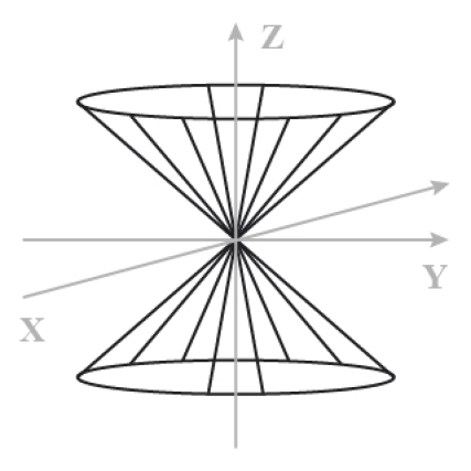
This figure represents the spins precession movement which is induced by the field Bo. For example, we may consider the proton as a magnetic dipole whose component µz is either parallel or anti parallel to the z axis. The angular speed of the precession moment is

The rotating coordinates or rotating frame

It is convenient to figure only the magnetic momentum of the excess of the nuclei in their fundamental states (Figure \(\PageIndex{1}\)).

Figure \(\PageIndex{2}\): The magnetization M in the rotating frame K’.

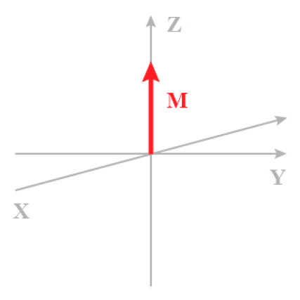
M is the macroscopic magnetization as a result of the individual nuclear moment µ. The xy plane does not contain any magnetization component. In addition to the coordinate system K(x,y,z), another system K'(x,y,z) rotates around the z axis with the angular speed thus . In this figure, is a virtual field B_f opposite to Bo, which is generated by the only relative rotation from one versus the other of the two coordinate systems K and K'. This means that the µ vector is static in the system K’ which is called rotating frame, it happens when has the same sign and the same value than 0. (3)

Requirements to get a resonance

The excitation of the nucleus is generated by a high frequency impulsion B₁ at a high power (50 watts) for a short time (10 to 50 µs). The field B_o is high and constant, the field B₁ is assumed to be weak, perpendicular to B₀ and rotates in the plane X_OY with an angular speed 1 and in the same sense than µ [3].

Practically, a small coil put perpendicular in the field B_o is run by a current (Figure \(\PageIndex{4}\)). This one causes an oscillatory induction along the axis of the coil. We may represent this induction Bx with two magnetic vectors rotating in opposite sense B(l) and B(r), one of which has the same rotation sense than the precession. The second vector is practically without any influence on the phenomenon.

The emitter coil on the x axis generates a weak electromagnetic field B₁ linearly polarized with a frequency and with an amplitude 2B₁.

Figure \(\PageIndex{4}\): Requirements for the resonance condition.

The Fourier Transform

We may compare the NMR spectroscopy and the optic one. In the optical spectroscopy, the prism allows the monochromatic analysis of a polychromatic source interacting with the mater. In the NMR spectroscopy, the impulsion B₁ yield a broad frequency spectrum and the Fourier transform allows a "monochromatic" analysis of the interaction beam/nucleus. The technique is to treat the signal M(t) according to the following relationship (2):

\[F(v)=\int_{0}^{\infty} f(t) \exp (-2 i \pi v t) d t \nonumber \]

Since the pulse sequence last generally less than a second, we may achieve a great number of accumulations of data before to proceed to the Fourier transform. The signal to noise ratio thus improves (this ratio is proportional to where S = number of scans).

Bibliography

1. La détection inverse en RMN ; M Boudonneu Analusis N°1, vol.18, 1990
2. La RMN concepts et méthodes; D. Canet inter éditions 1991
3. La spectroscope de RMN, H. Gunther MASSON 1994.
4. NMR in protein studies. M. P. Williamson. Chem. in Britain April 1991(335-337).
5. RMN 2D BRUKER 1993 Poly. 1, 2 et 3.
6. Resonance Magnétique Nucléaire; Evolution instrumentale et analyse de structure; J.P. Girault le technoscope de biofutur n°38 sept 90
7. Sensitivity enhancement by signal averaging in pulsed by Fourier transform NMR spectroscopy; D. L.Rabenteck; J. of Chem. Ed. Vol. 61, n°70, Oct 1984
8. Sequence Cosy Poly. BRUKER 1993.
9. Topic in chemical instrumentation part 3 and 4. 2 D Methods W. King and K. R. Williams J. of Chem. Educ. vol.67n°4.
10. Topics in chemical instrumentation (Definition) W. King and K. R. Williams
11. Two Dimensional NMR spectroscopy; Applications for chemists and biochemists; W. R. Crousmum, R. M. K. Carlson. Vol 9.
12. Two dimensional NMR Aspect 2000 - 3000 BRUKER
13. G. E. Reeman et Moms, J. ChemSoc, Chem.Comm, 684 (1978).
14. H. Kessler, W. Bernel and C. Giresinger, J. AM. Chem. Soc. 107, 1083 (1985).