By the late 19th century, many physicists thought their discipline was well on the way to explaining most natural phenomena. They could calculate the motions of material objects using Newton’s laws of classical mechanics, and they could describe the properties of radiant energy using mathematical relationships known as Maxwell’s equations, developed in 1873 by James Clerk Maxwell, a Scottish physicist. The universe appeared to be a simple and orderly place, containing matter, which consisted of particles that had mass and whose location and motion could be accurately described, and electromagnetic radiation, which was viewed as having no mass and whose exact position in space could not be fixed. Thus matter and energy were considered distinct and unrelated phenomena. Soon, however, scientists began to look more closely at a few inconvenient phenomena that could not be explained by the theories available at the time.
The traditional introduction to quantum mechanics involves discussing the breakdown of classical mechanics and where quantum steps in. We have three examples of this: (1) blackbody radiation, (2) photoelectric effect and (3) hydrogen emission (of light). We discuss them here.
First Evidence of Classical Breakdown: Blackbody Radiation
It has been known for a long time that hot things radiate light!
Figure \(\PageIndex{1}\): Blackbody Radiation. When heated, all objects emit electromagnetic radiation whose wavelength (and color) depends on the temperature of the object. A relatively low-temperature object, such as a horseshoe forged by a blacksmith, appears red, whereas a higher-temperature object, such as the surface of the sun, appears yellow or white. Images used with permission from Wikipedia.
Blackbody Radiators
To begin analyzing heat radiation, we need to be specific about the body doing the radiating: the simplest possible case is an idealized body which is a perfect absorber, and therefore also (from the above argument) a perfect emitter. For obvious reasons, this is called a “blackbody”. It is an idealized physical body that absorbs all incident electromagnetic radiation, regardless of frequency or angle of incidence.
Figure \(\PageIndex{2}\): A cavity with a small hole that approximates a physical blackbody radiator. Images used with permission via MIT .
A blackbody radiator is an object or system that absorbs all radiation incident upon it and re-radiates energy which is characteristic of only the radiating system only, not on the type of radiation which is incident upon it.
A physical realization of a blackbody is a cavity with a small hole with many reflections and absorptions. Very few entering photons (light rays) will get out. The inside of the cavity has radiation which is homogeneous and isotropic (the same in any direction, uniform everywhere).
Two experimental "laws" connected to black-body radiation:
Stefan-Boltzmann Law: The total (i.e., integrated) radiation intensity varies as \(T^4\). That is \[\int \text{all emitted light}\, d\nu \propto T^4\]
Note
The symbol \(\propto \) means "it is proportional to"
Wien’s Displacement Law: As the temperature of a blackbody varies, so does the frequency at which the emitted radiation is most intense. In fact, that frequency is directly proportional to the absolute temperature: \[\nu_{max} \propto T \label{-1}\]
where the proportionality constant is \(5.879 \times 10^{10} Hz/K\).
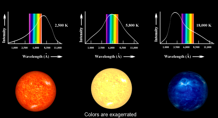
The concept underlying Equation \(\ref{-1}\) is familiar to most people. When an iron is heated in a fire, the first visible radiation (at around 900 K) is deep red, the lowest frequency visible light. Further increase in T causes the color to change to orange then yellow, and finally blue at very high temperatures (10,000 K or more) for which the peak in radiation intensity has moved beyond the visible into the ultraviolet (Figure \(\PageIndex{3}\)).
Figure \(\PageIndex{3}\): To estimate the surface temperature of a star, we can use the known relationship between the temperature of a blackbody, and the wavelength of light where its spectrum peaks (Equation \ref{-1}). That is, as you increase the temperature of a blackbody, the peak of its spectrum moves to shorter (bluer) wavelengths of light. This is illustrated where the intensity of three hypothetical stars is plotted against wavelength. The "rainbow" indicates the range of wavelengths that are visible to the human eye. (GNU 1.2; KStars Handbook).
Classic Blackbody Radiation
Lord Rayleigh and J. H. Jeans developed an equation which explained blackbody radiation at low frequencies.The equation which seemed to express blackbody radiation was built upon all the known assumptions of physics at the time.
The big assumption which Rayleigh and Jean implied was that infinitesimal amounts of energy were continuously added to the system when the frequency was increased.
Classical physics assumed that energy emitted by atomic oscillations could have any continuous value.This was true for anything that had been studied up until that point, including things like acceleration, position, or energy. The resulting Rayleigh-Jeans law was
Assumed that energy emitted by atomic oscillations could have any continuous value.
Aside: Distributions
Equation \(\ref{0}\) is a "distribution" not unlike the distribution of grades in a course. As such it has several properties of interest:
The integrated value (\(A\)): This is the sum over the distribution over all possible values of \(x\). Graphically, this is the area under the distribution. \[ A= \int_{-\infty}^{\infty} D(x)\, dx \label{1}\] If the range of \(x\) is less than \(-\infty\) to \(\infty\) (e.g., from \(a\) to \(b)\), then \(A\) is given by \[ A = \int_{a}^{b} D(x)\, dx \label{2}\]
The expectation value (\(\langle x \rangle \)): This is a different term that is used synonymously with the average (or mean) of \(x\) over the distribution. The mean is given by \[ \bar{x} = \langle x \rangle = \int_{a}^{b} x D(x)\, dx \label{3}\] Notice the difference between Equations \(\ref{2}\) and \(\ref{3}\).
The most probable value (\(x_{mp}\)): This is the value of \(x\) at the peak of \(D(x)\). This is determined from basic calculus for determining extrema and via identifying when the derivative of the distribution is zero. \[ \left( \dfrac{dD(x)}{dx} \right)_{x_{mp}} = 0 \label{4}\]
The standard deviation (\(\sigma_x\)): This is the a measure of the spread of the distribution and is given by \[ \sigma_x^2 = \int_{a}^{b} (x-\bar{x})^2 D(x) \,dx \label{5}\]
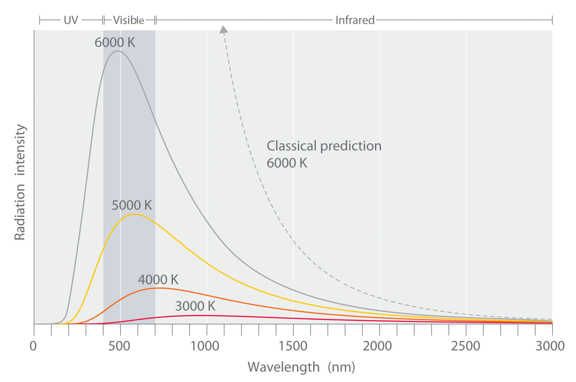
Experimental data performed on the black box showed slightly different results than what was expected by the Rayleigh-Jeans law.The law had been studied and widely accepted by many physicists of the day, but the experimental results did not lie, something was different between what was theorized and what actually happens.The experimental results showed a bell type of curve but according to the Rayleigh-Jeans law the frequency diverged as it neared the ultraviolet region (Equation \(\ref{0}\)). This inconsistency was termed the ultraviolet catastrophe.
Figure \(\PageIndex{1}\) Relationship between the Temperature of an Object and the Spectrum of Blackbody Radiation It Emits. At relatively low temperatures, most radiation is emitted at wavelengths longer than 700 nm, which is in the infrared portion of the spectrum. As the temperature of the object increases, the maximum intensity shifts to shorter wavelengths, successively resulting in orange, yellow, and finally white light. At high temperatures, all wavelengths of visible light are emitted with approximately equal intensities.
Max Planck was the first person to properly explain this experimental data. Rayleigh and Jean made the assumption that energy is continuous, but Planck took a slightly different approach. He said energy must come in certain unit intervals instead of being any random unit or number. He instead “quantized” energy in the form of
\[E= nh\nu\]
where \(n\) is an integer, \(h\) is a constant, and \(\nu\) is the frequency. This assumption proved to be the missing piece of the puzzle and Planck derived an expression which could explain the experimental data.
Max Planck proposed that energy is emitted in discrete packets - he didn't know what they were though.
From this, the Planck distribution law, with respect to frequency, was derived from
The resulting units of the radiant energy density function can be shown to be \(J \cdot m^{-3}\) by using the constants and their respective units.
By setting the wavelength \(\lambda\) = \(c \cdot \nu^{-1}\) and \(d\nu\) = \(c \cdot \dfrac {-d\lambda}{\lambda^2}\), you can express \(d\rho\) (\ref{Planck1}) in terms of \(\lambda\) rather than \(\nu\).
From this Equation \(\ref{10}\), it is clear that temperature and the maximum wavelength are inversely proportional. A larger temperature gives a smaller \(\lambda_{max}\), where a smaller temperature gives a larger \(\lambda_{max}\).
Interactive: Blackbody Spectrum
The mathematics implied that the energy given off by a blackbody was not continuous, but given off at certain specific wavelengths, in regular increments. If Planck assumed that the energy of blackbody radiation was in the form
\[E = nh \nu\]
where \(n\) is an integer (now called a quantum number), then he could explain what the mathematics represented.
The traditional introduction to quantum mechanics involves discussing the breakdown of classical mechanics and where quantum steps in.
Example \(\PageIndex{2}\): Calculating the Energy of Radiation
When we see light from a neon sign, we are observing radiation from excited neon atoms. If this radiation has a wavelength of 640 nm, what is the energy of the photon being emitted?
Solution
We use the part of Planck's equation that includes the wavelength, λ, and convert units of nanometers to meters so that the units of λ and c are the same.
The microwaves in an oven are of a specific frequency that will heat the water molecules contained in food. (This is why most plastics and glass do not become hot in a microwave oven-they do not contain water molecules.) This frequency is about 3 × 10⁹ Hz. What is the energy of one photon in these microwaves?
Answer
2 × 10⁻²⁴ J
Second Evidence of Classical Breakdown: The Photoelectric Effect
Ionization is the process by which an atom or a molecule acquires a negative or positive charge by gaining or losing electrons to form ions, often in conjunction with other chemical changes. You can read about the discussion of ionization energies.
Key to an electron ionization event is that energy is introduced and an electron is ejected.
There are different ways to add energy to systems (heat, electricity, bombarding of particles). Moreover, not only atoms, but molecules and bulk matter can be ionzed. The process we are interested in is injecting energy via the absorption of light, which is called the photoelectric effect.
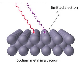
The photoelectric effect is the emission of electrons or other free carriers when light is shone onto a material. Electrons emitted in this manner can be called photo electrons.
Only five years after Planck’s proposed quantization, this hypothesis was used to explain a second phenomenon that conflicted with the accepted laws of classical physics. In 1886, the photoelectric effect was observed by Heinrich Hertz, by finding that when a metallic surface is exposed to ultraviolet light, electrons are emitted from the surface. When certain metals are exposed to light, electrons are ejected from their surface. Classical physics predicted that the number of electrons emitted and their kinetic energy should depend on only the intensity of the light, not its frequency.
The Photoelectric Effect involves the irradiating a metal surface with photons of sufficiently high energy to causes electrons to be ejected from the metal. (CC BY-SA-NC; anonymous by request).
Before delving into the photoelectric effect, let's discussing the the wave perspective of light and how it transfers energy.
The classical wave perspective of light and its associated Energy
Classical theory of light is a wave picture. Both amplitude and frequency are the two factors that affect the energy transferred by a wave: the height of the wave, and the number of waves passed by each second.
The amplitude tells you how much energy is in the wave. A high amplitude wave is a high-energy wave, and a low-amplitude wave is a low-energy wave. In the case of sound waves, a high amplitude sound will be loud, and a low amplitude sound will be quiet. Or with light waves, a high amplitude beam of light will be bright, and a low amplitude beam of light will be dim.
The other factor is frequency. Frequency is the number of waves that pass by each second, measured in hertz. So a wave of a particular amplitude will transmit more energy per second if it has a higher frequency, simply because more waves are passing by in a given period of time.
Classical Picture of Photoelectron Effect (Thermionic Emission)
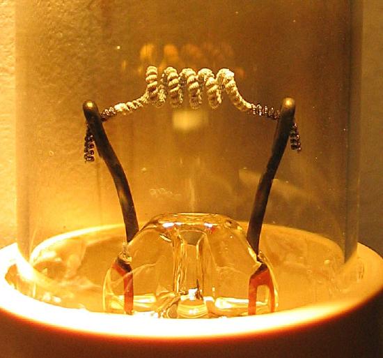
According to the classical perspective of photoelectric effect, when light shines on a surface, it slowly transfers energy into the substance. This increases the kinetic energy of the particles until finally, they give off excited electrons. This process is called Thermionic Emission and it was considered the most likely explanation for the photoelectric effect by physicists in in the early 20th century.
Thermionic Emission: Close up of the filament on a low pressure mercury gas discharge lamp showing white thermionic emission mix coating on the central portion of the coil. Typically made of a mixture of barium, strontium and calcium oxides, the coating is sputtered away through normal use, often eventually resulting in lamp failure. (CC-SA-BY 3.0; Deglr6328)
Expectations from Thermionic Emission based approach (The Classical Picture)
Increasing light intensity, regardless of frequency, would result in photoelectrons with higher kinetic energies
The photoelectric effect would not be observed immediately, since the substance must first reach a critical temperature before it can begin ejecting electrons.
Lenard's experimental setup. Image by Fowler. In the above figure, the battery represents the potential Lenard used to charge the collector plate negatively, which would actually be a variable voltage source. Since the electrons ejected by the blue light are getting to the collector plate, evidently the potential supplied by the battery is less than Vstop for blue light. Show with an arrow on the wire the direction of the electric current in the wire.
The applied voltage from the battery (\(V\)) is used to stop the electron from getting to the end. This is due to the energy of this applied field
\[E_{battery}= e V\]
matching or exceeding the kinetic energy of the photoelectrons
\[KE = \dfrac{1}{2} m v^2\]
On cranking up the negative voltage on the collector plate until the current just stops, that is, to \(V\), the highest kinetic energy electrons must have had energy \(eV\) on leaving the cathode.
Interactive: Five Key Experimental Results
Recreate the Lenard's experiment using the Photoelectric Effect simulation:
Below a certain threshold frequency, no matter how intense the light was, there was no emission of electrons.
Above the threshold frequency, the current (i.e. the # of electrons reaching the anode) was directly proportional to the light intensity.
The current appeared almost instantaneously after the light was turned on
Higher frequency light increased the kinetic energy of the electrons,
Changing the light intensity had no effect on the kinetic energy.
Higher frequencies may increase the energy of the ejected photoelectrons and make it cross a distance faster, but the time between each successive photoelectron remains the same because the time between each successive photon impact remains the same for the same intensity. It does not increase the total number of photoelectrons per photon.
Quantum Picture of the Photoelectron Effect
Einstein showed that the kinetic energy of the emitted electron depends on to the energy of the photon that hit the metallic surface and an effective "ionization energy" of the metal. This is shown by
\[ KE = \dfrac{mv^2}{2} = h\nu - \Phi \]
where \(\phi\) is the work function of the metal, and \(\phi\) = \(h\nu_0\), where \(\nu_0\) is the threshold frequency. However, each electron will only absorb the energy and be ejected if the frequency of the light is of sufficient energy according to the equation
\[ E = h\nu \]
where \(\nu\) is the frequency of the incident light and \(h\) is Planck's constant (\(h=6.626 \times 10^{-34} Js\)). The required energy to free an electron from an atom is called the work function and is designated by the symbol \(\phi\). The threshold frequency corresponds to a particle-light with the lowest energy needed to satisfy this work function (i.e. overcome the electron's affinity for the atom). Higher frequency light increases the kinetic energy (\(KE\)) of the ejected electron according to the equation:
\[ KE = h \nu - \Phi \label{6}\]
but it does not affect the number of photons ejected. To increase the number of electrons ejected, it is necessary to increase the number of photons (particle-light), since one photon is absorbed for each ejected electron.
Table 1 summarizes the work functions for several elements:
Table 1: Work Functions of Select Elements
Element
Work function Φ (eV)
Ionization Energy (eV)
Silver (Ag)
4.64
7.57
Aluminum (Al)
4.20
5.98
Gold (Au)
5.17
9.22
Boron (B)
4.45
8.298
Beryllium (Be)
4.98
9.32
Workfunctions and Ionization Energies are Different Concepts
In a particular textbook, the work function of a metal (in the context of the photoelectric effect) is defined as:
the minimum amount of energy necessary to remove an electron from the surface of the metal
the amount of energy required to remove an electron from an atom or molecule in the gaseous state
These two energies are generally different (Table 1). For instance, Copper has a work function of about 4.7 eV but has a higher ionization energy of about 746 kJ mol-1 or 7.7 eV.
Work function deals with "free" electrons in the metallic bonding of the metal, while ionization energy addressed the valence electrons still bound within the atom. Is the difference due to the energy required to overcome the attraction of the positive nucleus?
Ramifications of Einstein's Photon Theory of the Photoelectron effect
Since every photon of sufficient energy excites only one electron, increasing the light's intensity (i.e. the number of photons/sec) only increases the number of released electrons and not their kinetic energy.
No time is necessary for the atom to be heated to a critical temperature and therefore the release of the electron is nearly instantaneous upon absorption of the light.
The photons must be above a certain energy \( h \nu \geq h \nu_0\) to equal or exceed the workfunction, a threshold frequency exists below which no photoelectrons are observed.
Einstein's simple explanation completely accounted for the observed phenomenon in Lenard's experiment and began an investigation into the field we now call quantum mechanics. This new field seeks to provide a quantum explanation for classical mechanics and create a more unified theory of physics and thermodynamics. The study of the photoelectric effect has also lead to the creation of new photoelectron spectroscopy theory and applications.
In 1911 R. A. Milliken measured the value of \h (R. A. Millikan, Physical Review, Vol. 7, Issue 3, March 1916, pp. 355-388) obtaining a value of (\(h=6.57 \times 10^{-34} Js\)), only a 0.85% error with respect to the currently accepted value of (\(h=6.626 \times 10^{-34} Js\)).
The photoelectric effect concludes two important points
Photons are quantized, packets of energy.
Different metals have different work functions and threshold frequencies.
Third Evidence of Classical Breakdown: Atomic Spectra
Most of what is known about atomic (and molecular) structure and mechanics has been deduced from spectroscopy. A continuous spectrum can be produced by an incandescent solid or gas at high pressure. Blackbody radiation, for example, is a continuum since the degree of quantization from Planck's assumptions is so small the radiation curves look continuous (with other factors discussed later). An emission spectrum can be produced by a gas at low pressure excited by heat or by collisions with electrons. http://physics.bu.edu/~duffy/HTML5/emission_spectra.html or https://www.edumedia-sciences.com/en/media/661-emission-and-absorption-spectra
Continuous spectrum and two types of line spectra. from Wikipedia.
Interactive Element
Show emission spectrum for:
This is a simulation of the light emitted by excited gas atoms of particular elements. In some sense, these are atomic fingerprints. Note that the lines shown are the brightest lines in a spectrum - you may be able to see additional lines if you look at the spectrum from a real gas tube. In addition, the observed color could be a bit different from what is shown here. The visible spectrum is always shown as a reference.
Simulation first posted on 2-8-2017. Written by Andrew Duffy
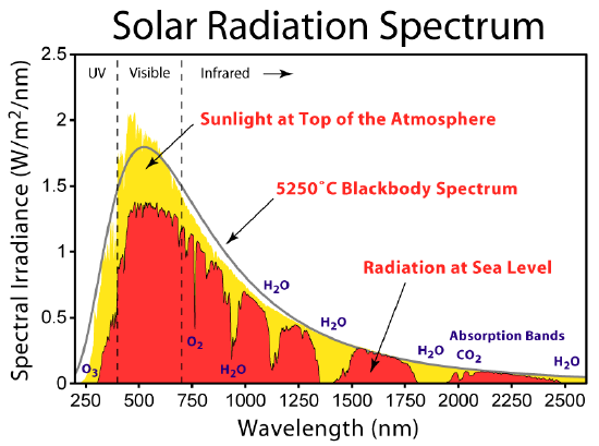
An absorption spectrum results when light from a continuous source passes through a cooler gas, consisting of a series of dark lines characteristic of the composition of the gas. Frauenhofer between 1814 and 1823 discovered nearly 600 dark lines in the solar spectrum viewed at high resolution. It is now understood that these lines are caused by absorption by the outer layers of the Sun and the Earth's atmosphere.
This figure shows the solar radiation spectrum for direct light at both the top of the Earth's atmosphere and at sea level. The sun produces light with a distribution similar to what would be expected from a 5525 K (5250 °C) blackbody, which is approximately the sun's surface temperature. As light passes through the atmosphere, some is absorbed by gases with specific absorption bands. from Wikipedia.
Gases heated to incandescence were found by Bunsen, Kirkhoff and others to emit light with a series of sharp wavelengths. The emitted light analyzed by a spectrometer (or even a simple prism) appears as a multitude of narrow bands of color. These so called line spectra are characteristic of the atomic composition of the gas.
(a) A sample of excited hydrogen atoms emits a characteristic red light. (b) When the light emitted by a sample of excited hydrogen atoms is split into its component wavelengths by a prism, four characteristic violet, blue, green, and red emission lines can be observed, the most intense of which is at 656 nm.
Experimental Observations (Hydrogen Gas)
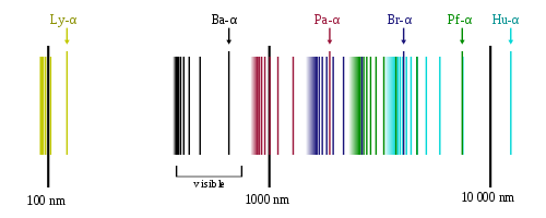
The line spectrum of hydrogen atoms is shown below.
The spectral series of hydrogen, on a logarithmic scale. (CC BY Sa 3.0; OrangeDog);
The hydrogen spectrum is complex, comprising more than the three lines visible to the naked eye. It is possible to detect patterns of lines in both the ultraviolet and infrared regions of the spectrum as well. These fall into a number of "series" of lines named after the person who discovered them.
Lyman series: λ, vacuum (nm)
Balmer series: λ, vacuum (nm)
Paschen series: λ, vacuum (nm)
Brackett series: λ, vacuum (nm)
Pfund series: λ, vacuum (nm)
Humphreys : λ, vacuum (nm)
121.57
656.3
1875
1875
7460
12.37
102.57
486.1
1282
1282
4654
7.503
97.254
434.0
1094
1094
3741
5.908
94.974
410.2
1005
1005
3297
5.129
93.780
397.0
954.6
954.6
3039
4.673
91.175
364.6
922.9
922.9
2279
3.282
Three particular series are well observed in emission of hydrogen atoms
The Lyman series (UV)
The Balmer series (Visible)
The Paschen series for (NIR)
The series can be phenomenologically described via the following relationships
\(\widetilde {\nu}\) is called the wavenumber (\(\widetilde{\nu}\)) and is the number of waves that fit in one unit of length (typically cm). This constant is named after the Swedish physicist Rydberg who (in 1888) presented a generalization of formulas identified for the specific series (Equations \ref{2.1} - \ref{2.3}).
For the Lyman series, \(n_1=1\) and \(n_2\) varies from 2 to \(\infty\).
For the Balmer series, \(n_1 = 2\) and \(n_2\) varies from 3 to \(\infty\).
For the Paschen series, \(n_1 = 3\) and \(n_2\) varies from 4 to \(\infty\).
For each series, when \(n_2\) approaches \(\infty\), \(\widetilde {\nu}\) gets bigger and the lines become more dense (i.e., more lines per wavenumber). Furthermore, \widetilde {\nu} will reach an asymptotic value:
and since \(\widetilde {\nu}\) = \(\dfrac {1}{\lambda}\), \(\lambda\) gets successively smaller as \(n_2\) increases.
But what do \(n_1\) and \(n_2\) represent?
Rydberg suggested that all atomic spectra formed families with pattern given by Equation \ref{2.4}. It turns out that there are families of spectra following Rydberg's pattern, notably in the alkali metals, sodium, potassium, etc., but not with the precision the hydrogen atom lines fit the formula in Equations \ref{2.1} - \ref{2.3}, and low values of \(n_1\) give lines that deviate considerably. As we will discuss extensively later on this is if because there are more than one electron in these systems.
Summary
Electromagnetic radiation demonstrates properties of particles called photons. The energy of a photon is related to the frequency (or alternatively, the wavelength) of the radiation as E = hν (or \(E=\dfrac{hc}{λ}\)), where h is Planck's constant. That light demonstrates both wavelike and particle-like behavior is known as wave-particle duality. All forms of electromagnetic radiation share these properties, although various forms including X-rays, visible light, microwaves, and radio waves interact differently with matter and have very different practical applications. Electromagnetic radiation can be generated by exciting matter to higher energies, such as by heating it. The emitted light can be either continuous (incandescent sources like the sun) or discrete (from specific types of excited atoms).