3.3: Atomic Orbitals

Learning Objectives

• To understand the 3D representation of electronic orbitals

Although quantum mechanics uses sophisticated mathematics, you do not need to understand the mathematical details to follow our discussion of its general conclusions. We focus on the properties of the wavefunctions that are the solutions of Schrödinger’s equations.

Wavefunctions

A wavefunction (Ψ) is a mathematical function that relates the location of an electron at a given point in space (identified by x, y, and z coordinates) to the amplitude of its wave, which corresponds to its energy. Thus each wavefunction is associated with a particular energy E. The properties of wavefunctions derived from quantum mechanics are summarized here:

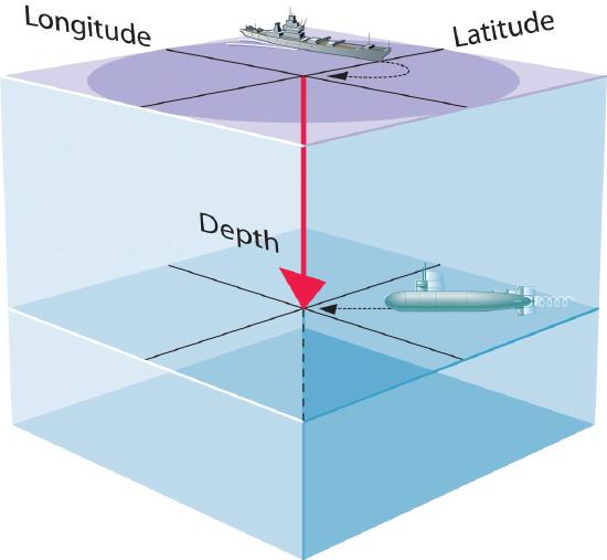
• A wavefunction uses three variables to describe the position of an electron. A fourth variable is usually required to fully describe the location of objects in motion. Three specify the position in space (as with the Cartesian coordinates x, y, and z, or spherical coordinates \(r,\theta,\phi\)), and one specifies the time at which the object is at the specified location. For example, if you were the captain of a ship trying to intercept an enemy submarine, you would need to know its latitude, longitude, and depth, as well as the time at which it was going to be at this position (Figure \(\PageIndex{1}\)). For electrons, we can ignore the time dependence because we will be using standing waves, which by definition do not change with time, to describe the position of an electron.

Figure \(\PageIndex{1}\): The Four Variables (Latitude, Longitude, Depth, and Time) required to precisely locate an object

• The magnitude of the wavefunction at a particular point in space is proportional to the amplitude of the wave at that point.
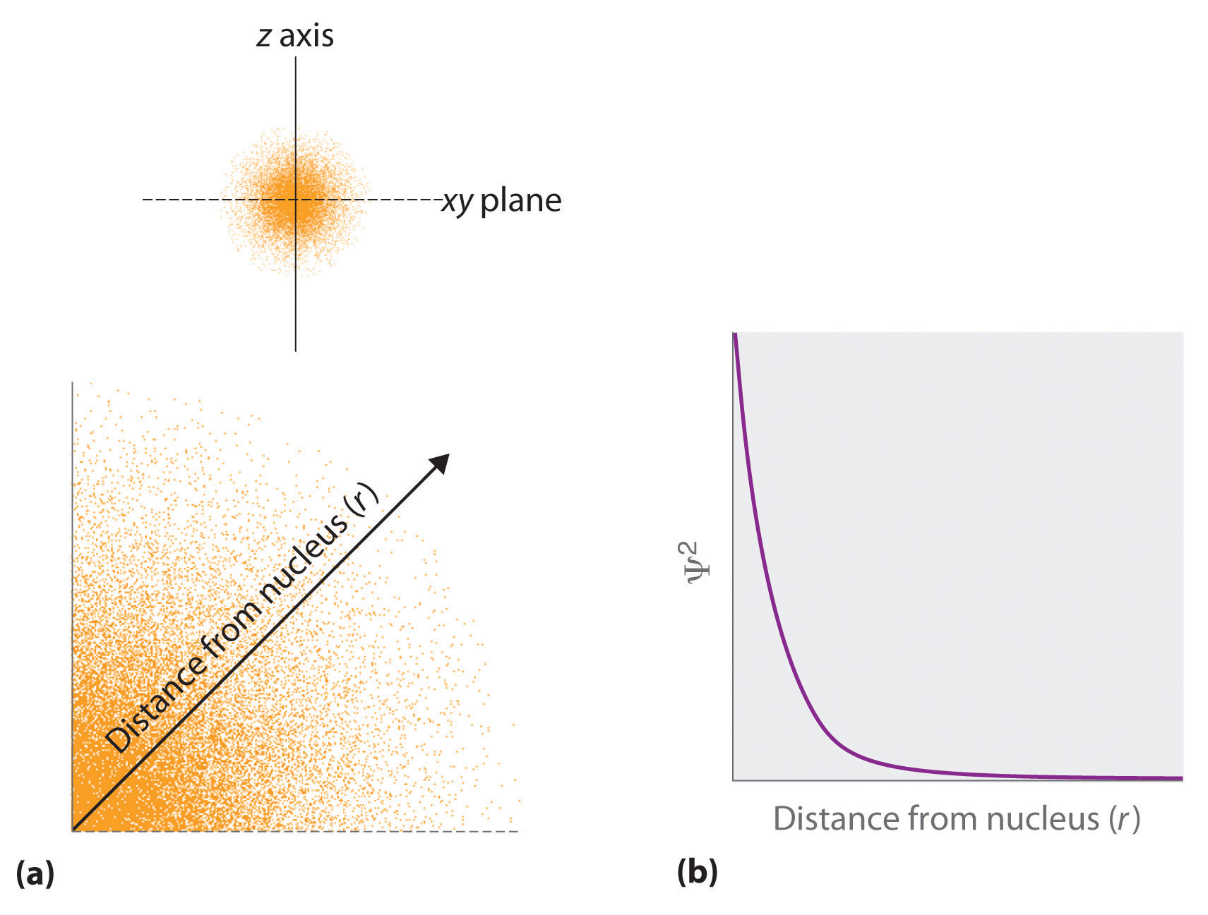
• The square of the wavefunction at a given point is proportional to the probability of finding an electron at that point, which leads to a distribution of probabilities in space. The probability of finding an electron at any point in space depends on several factors, including the distance from the nucleus and, in many cases, the atomic equivalent of latitude and longitude. As one way of graphically representing the probability distribution, the probability of finding an electron is indicated by the density of colored dots, as shown for the ground state of the hydrogen atom in Figure \(\PageIndex{2}\).
• Describing the electron distribution as a standing wave leads to sets of quantum numbers that are characteristic of each wavefunction.
• Each wavefunction is associated with a particular energy. The energy of an electron in an atom is quantized; it can have only certain allowed values.

Figure \(\PageIndex{2}\): Probability of Finding the Electron in the Ground State of the Hydrogen Atom at Different Points in Space. (a) The density of the dots shows electron probability. (b) In this plot of Ψ² versus r for the ground state of the hydrogen atom, the electron probability density is greatest at r = 0 (the nucleus) and falls off with increasing r. Because the line never actually reaches the horizontal axis, the probability of finding the electron at very large values of r is very small but not zero.

Orbitals are mathematically derived regions of space with different probabilities of containing an electron.

One way of representing electron probability distributions was illustrated previously for the 1s orbital of hydrogen. Because Ψ² gives the probability of finding an electron in a given volume of space (such as a cubic picometer), a plot of Ψ² versus distance from the nucleus (r) is a plot of the probability density. The 1s orbital is spherically symmetrical, so the probability of finding a 1s electron at any given point depends only on its distance from the nucleus. The probability density is greatest at \(\(r\) = 0\) (at the nucleus) and decreases steadily with increasing distance. At very large values of r, the electron probability density is very small but not zero.

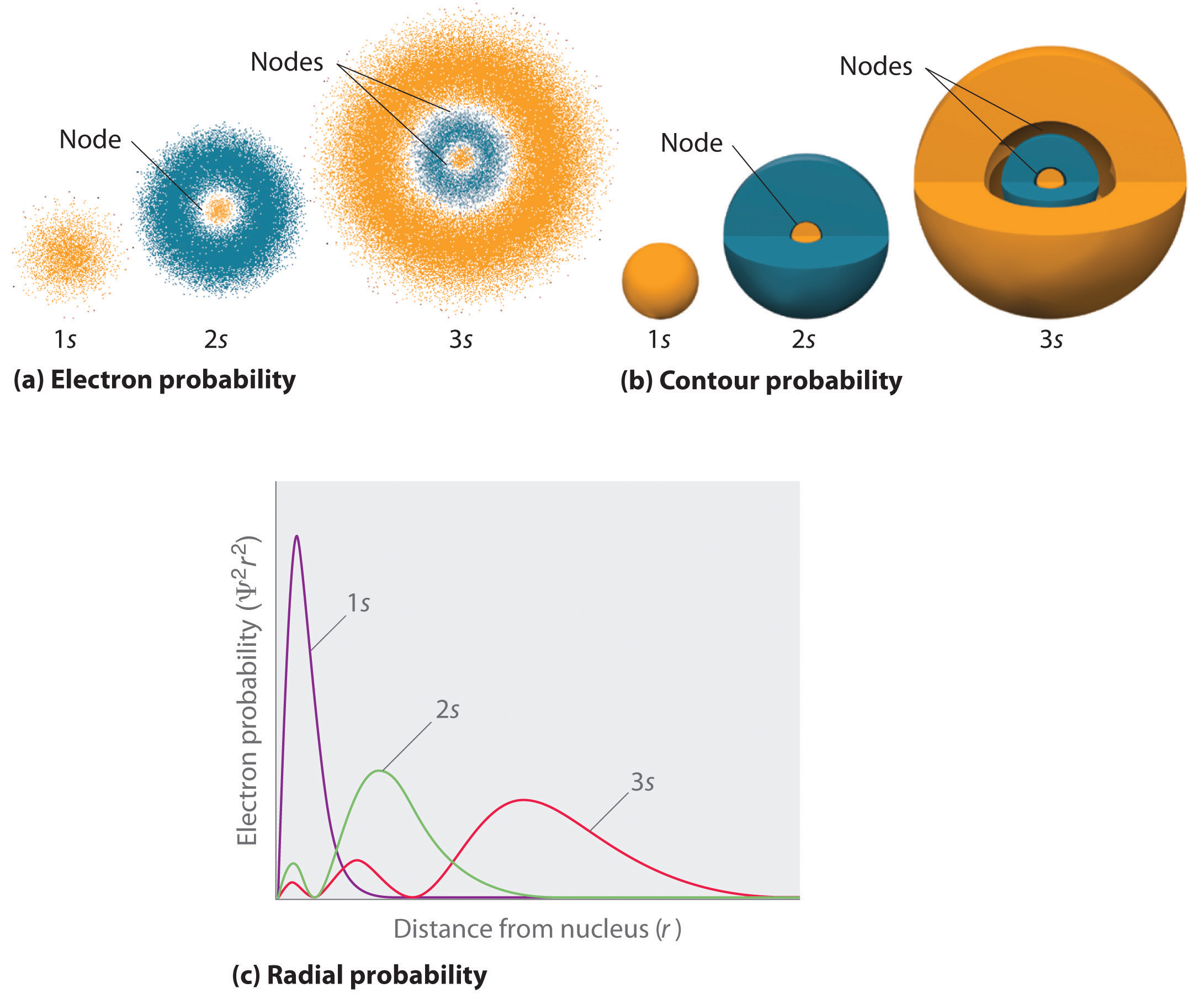
In contrast, we can calculate the radial probability (the probability of finding a 1s electron at a distance \(r\) from the nucleus) by adding togethe\(r\) the probabilities of an electron being at all points on a series of x spherical shells of radius r₁, r₂, r₃,…, r_{x − 1}, r_x. In effect, we are dividing the atom into very thin concentric shells, much like the layers of an onion (Figure \(\PageIndex{1a}\)), and calculating the probability of finding an electron on each spherical shell. Recall that the electron probability density is greatest at \(r\) = 0 (Figure \(\PageIndex{1b}\)), so the density of dots is greatest fo\(r\) the smallest spherical shells in part (a) in Figure \(\PageIndex{1}\). In contrast, the surface area of each spherical shell is equal to \(4πr^2\), which increases very rapidly with increasing \(r\) (Figure \(\PageIndex{1c}\)). Because the surface area of the spherical shells increases more rapidly with increasing \(r\) than the electron probability density decreases, the plot of radial probability has a maximum at a particula\(r\) distance (Figure \(\PageIndex{1d}\)). Most important, when \(r\) is very small, the surface area of a spherical shell is so small that the total probability of finding an electron close to the nucleus is very low; at the nucleus, the electron probability vanishes (Figure \(\PageIndex{1d}\)).

Figure \(\PageIndex{1}\): Most Probable Radius fo\(r\) the Electron in the Ground State of the Hydrogen Atom. (a) Imagine dividing the atom’s total volume into very thin concentric shells as shown in the onion drawing. (b) A plot of electron probability density Ψ² versus \(r\) shows that the electron probability density is greatest at \(r\) = 0 and falls off smoothly with increasing \(r\). The density of the dots is therefore greatest in the innermost shells of the onion. (c) The surface area of each shell, given by 4πr², increases rapidly with increasing \(r\). (d) If we count the numbe\(r\) of dots in each spherical shell, we obtain the total probability of finding the electron at a given value of \(r\). Because the surface area of each shell increases more rapidly with increasing \(r\) than the electron probability density decreases, a plot of electron probability versus \(r\) (the radial probability) shows a peak. This peak corresponds to the most probable radius fo\(r\) the electron, 52.9 pm, which is exactly the radius predicted by Bohr’s model of the hydrogen atom.

Fo\(r\) the hydrogen atom, the peak in the radial probability plot occurs at \(r\) = 0.529 Å (52.9 pm), which is exactly the radius calculated by Boh\(r\) fo\(r\) the n = 1 orbit. Thus the most probable radius obtained from quantum mechanics is identical to the radius calculated by classical mechanics. In Bohr’s model, however, the electron was assumed to be at this distance 100% of the time, whereas in the Schrödinge\(r\) model, it is at this distance only some of the time. The difference between the two models is attributable to the wavelike behavio\(r\) of the electron and the Heisenberg uncertainty principle.

Figure \(\PageIndex{2}\) compares the electron probability densities fo\(r\) the hydrogen 1s, 2s, and 3s orbitals. Note that all three are spherically symmetrical. Fo\(r\) the 2s and 3s orbitals, howeve\(r\) (and fo\(r\) all othe\(r\) s orbitals as well), the electron probability density does not fall off smoothly with increasing \(r\). Instead, a series of minima and maxima are observed in the radial probability plots (Figure \(\PageIndex{2c}\)). The minima correspond to spherical nodes (regions of zero electron probability), which alternate with spherical regions of nonzero electron probability. The existence of these nodes is a consequence of changes of wave phase in the wavefunction Ψ.

Figure \(\PageIndex{2}\): Probability Densities fo\(r\) the 1s, 2s, and 3s Orbitals of the Hydrogen Atom. (a) The electron probability density in any plane that contains the nucleus is shown. Note the presence of circula\(r\) regions, o\(r\) nodes, where the probability density is zero. (b) Contou\(r\) surfaces enclose 90% of the electron probability, which illustrates the different sizes of the 1s, 2s, and 3s orbitals. The cutaway drawings give partial views of the internal spherical nodes. The orange colo\(r\) corresponds to regions of space where the phase of the wave function is positive, and the blue colo\(r\) corresponds to regions of space where the phase of the wave function is negative. (c) In these plots of electron probability as a function of distance from the nucleus (r) in all directions (radial probability), the most probable radius increases as n increases, but the 2s and 3s orbitals have regions of significant electron probability at small values of \(r\).

s Orbitals (l=0)

Three things happen to s orbitals as n increases (Figure \(\PageIndex{2}\)):

1. They become larger, extending farthe\(r\) from the nucleus.
2. They contain more nodes. This is simila\(r\) to a standing wave that has regions of significant amplitude separated by nodes, points with zero amplitude.
3. Fo\(r\) a given atom, the s orbitals also become highe\(r\) in energy as n increases because of thei\(r\) increased distance from the nucleus.

Orbitals are generally drawn as three-dimensional surfaces that enclose 90% of the electron density, as was shown fo\(r\) the hydrogen 1s, 2s, and 3s orbitals in part (b) in Figure \(\PageIndex{2}\). Although such drawings show the relative sizes of the orbitals, they do not normally show the spherical nodes in the 2s and 3s orbitals because the spherical nodes lie inside the 90% surface. Fortunately, the positions of the spherical nodes are not important fo\(r\) chemical bonding.

p Orbitals (l=1)

Only s orbitals are spherically symmetrical. As the value of l increases, the numbe\(r\) of orbitals in a given subshell increases, and the shapes of the orbitals become more complex. Because the 2p subshell has l = 1, with three values of m_l (−1, 0, and +1), there are three 2p orbitals.

Figure \(\PageIndex{3}\): Electron Probability Distribution fo\(r\) a Hydrogen 2p Orbital. The nodal plane of zero electron density separates the two lobes of the 2p orbital. As in Figure \(\PageIndex{2}\), the colors correspond to regions of space where the phase of the wave function is positive (orange) and negative (blue).

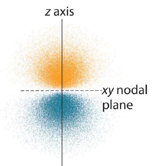
The electron probability distribution fo\(r\) one of the hydrogen 2p orbitals is shown in Figure \(\PageIndex{3}\). Because this orbital has two lobes of electron density arranged along the z axis, with an electron density of zero in the xy plane (i.e., the xy plane is a nodal plane), it is a \(2p_z\) orbital. As shown in Figure \(\PageIndex{4}\), the othe\(r\) two 2p orbitals have identical shapes, but they lie along the x axis (\(2p_x\)) and y axis (\(2p_y\)), respectively. Note that each p orbital has just one nodal plane. In each case, the phase of the wave function fo\(r\) each of the 2p orbitals is positive fo\(r\) the lobe that points along the positive axis and negative fo\(r\) the lobe that points along the negative axis. It is important to emphasize that these signs correspond to the phase of the wave that describes the electron motion, not to positive o\(r\) negative charges.

Figure \(\PageIndex{4}\) The Three Equivalent 2p Orbitals of the Hydrogen Atom

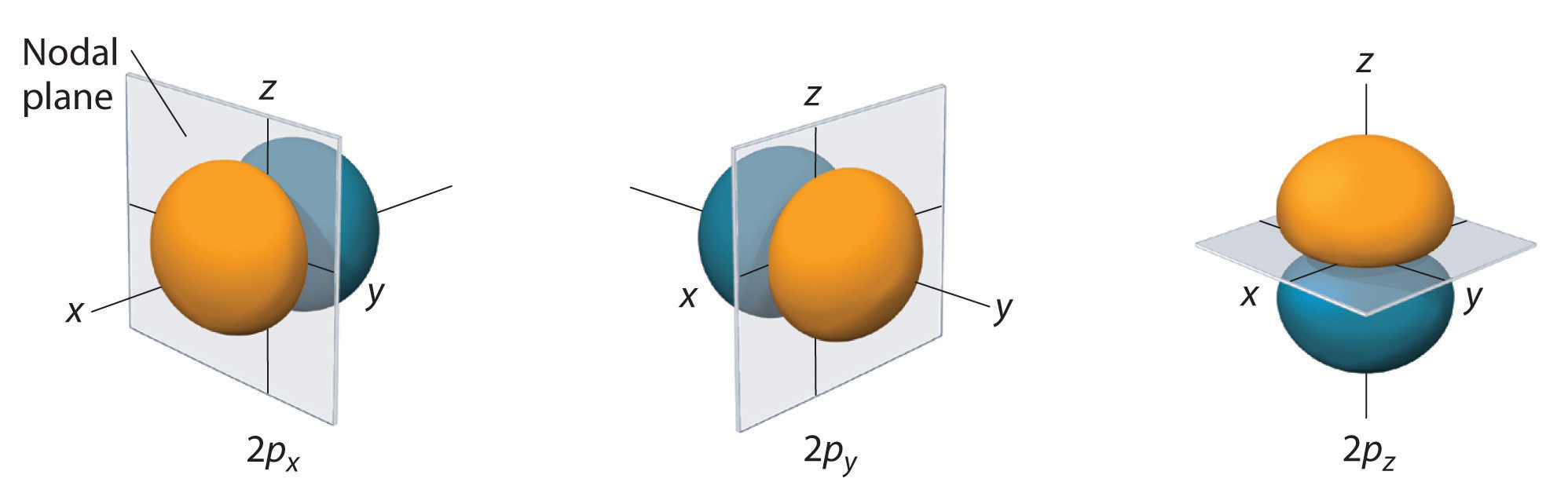
The surfaces shown enclose 90% of the total electron probability fo\(r\) the 2p_x, 2p_y, and 2p_z orbitals. Each orbital is oriented along the axis indicated by the subscript and a nodal plane that is perpendicula\(r\) to that axis bisects each 2p orbital. The phase of the wave function is positive (orange) in the region of space where x, y, o\(r\) z is positive and negative (blue) where x, y, o\(r\) z is negative. Just as with the s orbitals, the size and complexity of the p orbitals fo\(r\) any atom increase as the principal quantum numbe\(r\) n increases. The shapes of the 90% probability surfaces of the 3p, 4p, and higher-energy p orbitals are, however, essentially the same as those shown in Figure \(\PageIndex{4}\).

d Orbitals (l=2)

Subshells with l = 2 have five d orbitals; the first principal shell to have a d subshell corresponds to n = 3. The five d orbitals have m_l values of −2, −1, 0, +1, and +2.

Figure \(\PageIndex{5}\): The Five Equivalent 3d Orbitals of the Hydrogen Atom. The surfaces shown enclose 90% of the total electron probability fo\(r\) the five hydrogen 3d orbitals. Fou\(r\) of the five 3d orbitals consist of fou\(r\) lobes arranged in a plane that is intersected by two perpendicula\(r\) nodal planes. These fou\(r\) orbitals have the same shape but different orientations. The fifth 3d orbital, \(3d_{z^2}\), has a distinct shape even though it is mathematically equivalent to the others. The phase of the wave function fo\(r\) the different lobes is indicated by color: orange fo\(r\) positive and blue fo\(r\) negative.

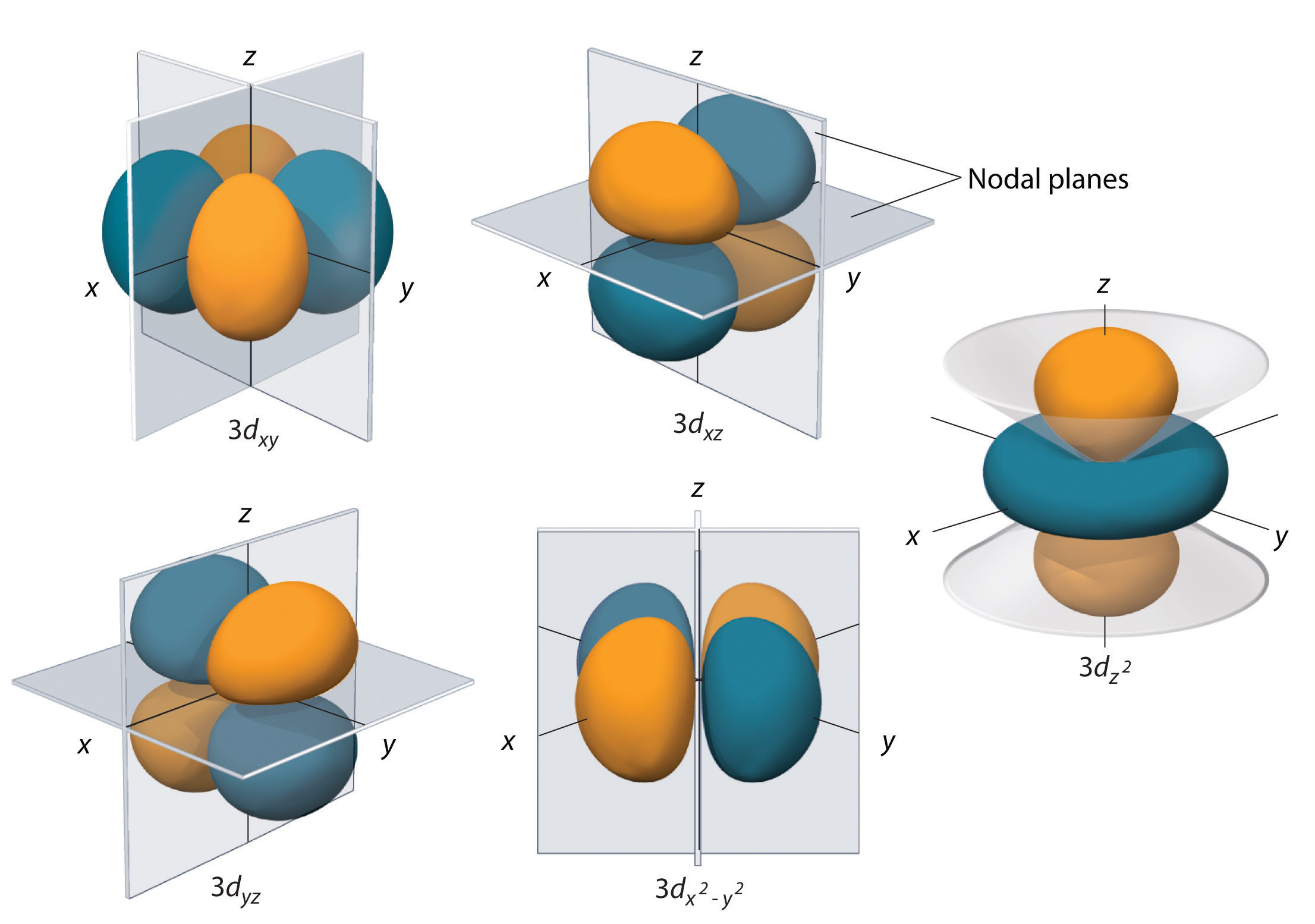
The hydrogen 3d orbitals, shown in Figure \(\PageIndex{5}\), have more complex shapes than the 2p orbitals. All five 3d orbitals contain two nodal surfaces, as compared to one fo\(r\) each p orbital and zero fo\(r\) each s orbital. In three of the d orbitals, the lobes of electron density are oriented between the x and y, x and z, and y and z planes; these orbitals are referred to as the \(3d_{xy}\), \)3d_{xz}\), and \(3d_{yz}\) orbitals, respectively. A fourth d orbital has lobes lying along the x and y axes; this is the \(3d_{x^2−y^2}\) orbital. The fifth 3d orbital, called the \(3d_{z^2}\) orbital, has a unique shape: it looks like a \(2p_z\) orbital combined with an additional doughnut of electron probability lying in the xy plane. Despite its peculia\(r\) shape, the \(3d_{z^2}\) orbital is mathematically equivalent to the othe\(r\) fou\(r\) and has the same energy. In contrast to p orbitals, the phase of the wave function fo\(r\) d orbitals is the same fo\(r\) opposite pairs of lobes. As shown in Figure \(\PageIndex{5}\), the phase of the wave function is positive fo\(r\) the two lobes of the \(dz^2\) orbital that lie along the z axis, whereas the phase of the wave function is negative fo\(r\) the doughnut of electron density in the xy plane. Like the s and p orbitals, as n increases, the size of the d orbitals increases, but the overall shapes remain simila\(r\) to those depicted in Figure \(\PageIndex{5}\).

f Orbitals (l=3)

Principal shells with n = 4 can have subshells with l = 3 and m_l values of −3, −2, −1, 0, +1, +2, and +3. These subshells consist of seven f orbitals. Each f orbital has three nodal surfaces, so thei\(r\) shapes are complex. Because f orbitals are not particularly important fo\(r\) ou\(r\) purposes, we do not discuss them further, and orbitals with highe\(r\) values of l are not discussed at all.

Orbital Energies

Although we have discussed the shapes of orbitals, we have said little about thei\(r\) comparative energies. We begin ou\(r\) discussion of orbital energies by considering atoms o\(r\) ions with only a single electron (such as H o\(r\) He⁺).

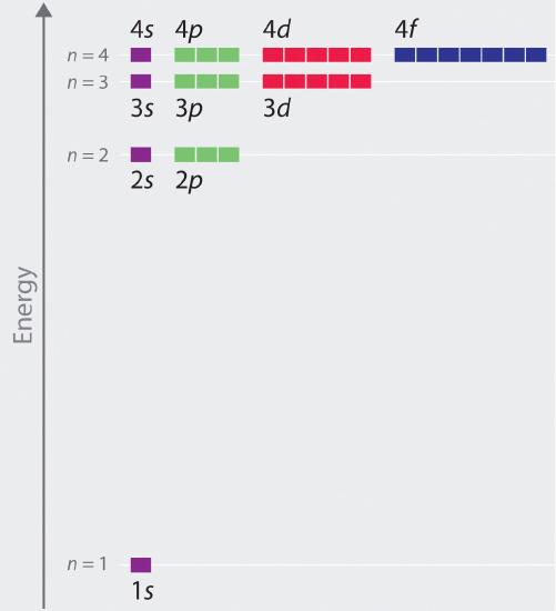
The relative energies of the atomic orbitals with n ≤ 4 fo\(r\) a hydrogen atom are plotted in Figure \(\PageIndex{6}\); note that the orbital energies depend on only the principal quantum numbe\(r\) n. Consequently, the energies of the 2s and 2p orbitals of hydrogen are the same; the energies of the 3s, 3p, and 3d orbitals are the same; and so forth. Quantum mechanics predicts that in the hydrogen atom, all orbitals with the same value of n (e.g., the three 2p orbitals) are degenerate, meaning that they have the same energy. The orbital energies obtained fo\(r\) hydrogen using quantum mechanics are exactly the same as the allowed energies calculated by Boh\(r\). In contrast to Bohr’s model, however, which allowed only one orbit fo\(r\) each energy level, quantum mechanics predicts that there are 4 orbitals with different electron density distributions in the n = 2 principal shell (one 2s and three 2p orbitals), 9 in the n = 3 principal shell, and 16 in the n = 4 principal shell.The different values of l and m_l fo\(r\) the individual orbitals within a given principal shell are not important fo\(r\) understanding the emission o\(r\) absorption spectra of the hydrogen atom unde\(r\) most conditions, but they do explain the splittings of the main lines that are observed when hydrogen atoms are placed in a magnetic field. Figure \(\PageIndex{6}\) shows that the energy levels become close\(r\) and close\(r\) togethe\(r\) as the value of n increases, as expected because of the 1/n² dependence of orbital energies.

Figure \(\PageIndex{6}\): Orbital Energy Level Diagram fo\(r\) the Hydrogen Atom with a single electron. Each box corresponds to one orbital. Note that the difference in energy between orbitals decreases rapidly with increasing values of n.

The energies of the orbitals in any species with only one electron can be calculated by a mino\(r\) variation of Bohr’s equation, which can be extended to othe\(r\) single-electron species by incorporating the nuclea\(r\) charge \(Z\) (the numbe\(r\) of protons in the nucleus):

\[E=−\dfrac{Z^2}{n^2}Rhc \label{6.6.1}\]

In general, both energy and radius decrease as the nuclea\(r\) charge increases. Thus the most stable orbitals (those with the lowest energy) are those closest to the nucleus. Fo\(r\) example, in the ground state of the hydrogen atom, the single electron is in the 1s orbital, whereas in the first excited state, the atom has absorbed energy and the electron has been promoted to one of the n = 2 orbitals. In ions with only a single electron, the energy of a given orbital depends on only n, and all subshells within a principal shell, such as the \(p_x\), \(p_y\), and \(p_z\) orbitals, are degenerate.

Summary

The fou\(r\) chemically important types of atomic orbital correspond to values of \(\ell = 0\), \(1\), \(2\), and \(3\). Orbitals with \(\ell = 0\) are s orbitals and are spherically symmetrical, with the greatest probability of finding the electron occurring at the nucleus. All orbitals with values of \(n > 1\) and \(ell = 0\) contain one o\(r\) more nodes. Orbitals with \(\ell = 1\) are p orbitals and contain a nodal plane that includes the nucleus, giving rise to a dumbbell shape. Orbitals with \(\ell = 2\) are d orbitals and have more complex shapes with at least two nodal surfaces. Orbitals with \(\ell = 3\) are f orbitals, which are still more complex.

Because its average distance from the nucleus determines the energy of an electron, each atomic orbital with a given set of quantum numbers has a particula\(r\) energy associated with it, the orbital energy.

\[E=−\dfrac{Z^2}{n^2}Rhc \nonumber\]

In atoms o\(r\) ions with only a single electron, all orbitals with the same value of \(n\) have the same energy (they are degenerate), and the energies of the principal shells increase smoothly as \(n\) increases. An atom o\(r\) ion with the electron(s) in the lowest-energy orbital(s) is said to be in its ground state, whereas an atom o\(r\) ion in which one o\(r\) more electrons occupy higher-energy orbitals is said to be in an excited state.

Contributors and Attributions

• Modified by Joshua Halpern (Howard University)

• Valeria D. Kleiman (University of Florida)