
4: Bohr atom and Heisenberg Uncertainty (Lecture)
- Page ID
- 38614
\( \newcommand{\vecs}[1]{\overset { \scriptstyle \rightharpoonup} {\mathbf{#1}} } \)
\( \newcommand{\vecd}[1]{\overset{-\!-\!\rightharpoonup}{\vphantom{a}\smash {#1}}} \)
\( \newcommand{\id}{\mathrm{id}}\) \( \newcommand{\Span}{\mathrm{span}}\)
( \newcommand{\kernel}{\mathrm{null}\,}\) \( \newcommand{\range}{\mathrm{range}\,}\)
\( \newcommand{\RealPart}{\mathrm{Re}}\) \( \newcommand{\ImaginaryPart}{\mathrm{Im}}\)
\( \newcommand{\Argument}{\mathrm{Arg}}\) \( \newcommand{\norm}[1]{\| #1 \|}\)
\( \newcommand{\inner}[2]{\langle #1, #2 \rangle}\)
\( \newcommand{\Span}{\mathrm{span}}\)
\( \newcommand{\id}{\mathrm{id}}\)
\( \newcommand{\Span}{\mathrm{span}}\)
\( \newcommand{\kernel}{\mathrm{null}\,}\)
\( \newcommand{\range}{\mathrm{range}\,}\)
\( \newcommand{\RealPart}{\mathrm{Re}}\)
\( \newcommand{\ImaginaryPart}{\mathrm{Im}}\)
\( \newcommand{\Argument}{\mathrm{Arg}}\)
\( \newcommand{\norm}[1]{\| #1 \|}\)
\( \newcommand{\inner}[2]{\langle #1, #2 \rangle}\)
\( \newcommand{\Span}{\mathrm{span}}\) \( \newcommand{\AA}{\unicode[.8,0]{x212B}}\)
\( \newcommand{\vectorA}[1]{\vec{#1}} % arrow\)
\( \newcommand{\vectorAt}[1]{\vec{\text{#1}}} % arrow\)
\( \newcommand{\vectorB}[1]{\overset { \scriptstyle \rightharpoonup} {\mathbf{#1}} } \)
\( \newcommand{\vectorC}[1]{\textbf{#1}} \)
\( \newcommand{\vectorD}[1]{\overrightarrow{#1}} \)
\( \newcommand{\vectorDt}[1]{\overrightarrow{\text{#1}}} \)
\( \newcommand{\vectE}[1]{\overset{-\!-\!\rightharpoonup}{\vphantom{a}\smash{\mathbf {#1}}}} \)
\( \newcommand{\vecs}[1]{\overset { \scriptstyle \rightharpoonup} {\mathbf{#1}} } \)
\( \newcommand{\vecd}[1]{\overset{-\!-\!\rightharpoonup}{\vphantom{a}\smash {#1}}} \)
\(\newcommand{\avec}{\mathbf a}\) \(\newcommand{\bvec}{\mathbf b}\) \(\newcommand{\cvec}{\mathbf c}\) \(\newcommand{\dvec}{\mathbf d}\) \(\newcommand{\dtil}{\widetilde{\mathbf d}}\) \(\newcommand{\evec}{\mathbf e}\) \(\newcommand{\fvec}{\mathbf f}\) \(\newcommand{\nvec}{\mathbf n}\) \(\newcommand{\pvec}{\mathbf p}\) \(\newcommand{\qvec}{\mathbf q}\) \(\newcommand{\svec}{\mathbf s}\) \(\newcommand{\tvec}{\mathbf t}\) \(\newcommand{\uvec}{\mathbf u}\) \(\newcommand{\vvec}{\mathbf v}\) \(\newcommand{\wvec}{\mathbf w}\) \(\newcommand{\xvec}{\mathbf x}\) \(\newcommand{\yvec}{\mathbf y}\) \(\newcommand{\zvec}{\mathbf z}\) \(\newcommand{\rvec}{\mathbf r}\) \(\newcommand{\mvec}{\mathbf m}\) \(\newcommand{\zerovec}{\mathbf 0}\) \(\newcommand{\onevec}{\mathbf 1}\) \(\newcommand{\real}{\mathbb R}\) \(\newcommand{\twovec}[2]{\left[\begin{array}{r}#1 \\ #2 \end{array}\right]}\) \(\newcommand{\ctwovec}[2]{\left[\begin{array}{c}#1 \\ #2 \end{array}\right]}\) \(\newcommand{\threevec}[3]{\left[\begin{array}{r}#1 \\ #2 \\ #3 \end{array}\right]}\) \(\newcommand{\cthreevec}[3]{\left[\begin{array}{c}#1 \\ #2 \\ #3 \end{array}\right]}\) \(\newcommand{\fourvec}[4]{\left[\begin{array}{r}#1 \\ #2 \\ #3 \\ #4 \end{array}\right]}\) \(\newcommand{\cfourvec}[4]{\left[\begin{array}{c}#1 \\ #2 \\ #3 \\ #4 \end{array}\right]}\) \(\newcommand{\fivevec}[5]{\left[\begin{array}{r}#1 \\ #2 \\ #3 \\ #4 \\ #5 \\ \end{array}\right]}\) \(\newcommand{\cfivevec}[5]{\left[\begin{array}{c}#1 \\ #2 \\ #3 \\ #4 \\ #5 \\ \end{array}\right]}\) \(\newcommand{\mattwo}[4]{\left[\begin{array}{rr}#1 \amp #2 \\ #3 \amp #4 \\ \end{array}\right]}\) \(\newcommand{\laspan}[1]{\text{Span}\{#1\}}\) \(\newcommand{\bcal}{\cal B}\) \(\newcommand{\ccal}{\cal C}\) \(\newcommand{\scal}{\cal S}\) \(\newcommand{\wcal}{\cal W}\) \(\newcommand{\ecal}{\cal E}\) \(\newcommand{\coords}[2]{\left\{#1\right\}_{#2}}\) \(\newcommand{\gray}[1]{\color{gray}{#1}}\) \(\newcommand{\lgray}[1]{\color{lightgray}{#1}}\) \(\newcommand{\rank}{\operatorname{rank}}\) \(\newcommand{\row}{\text{Row}}\) \(\newcommand{\col}{\text{Col}}\) \(\renewcommand{\row}{\text{Row}}\) \(\newcommand{\nul}{\text{Nul}}\) \(\newcommand{\var}{\text{Var}}\) \(\newcommand{\corr}{\text{corr}}\) \(\newcommand{\len}[1]{\left|#1\right|}\) \(\newcommand{\bbar}{\overline{\bvec}}\) \(\newcommand{\bhat}{\widehat{\bvec}}\) \(\newcommand{\bperp}{\bvec^\perp}\) \(\newcommand{\xhat}{\widehat{\xvec}}\) \(\newcommand{\vhat}{\widehat{\vvec}}\) \(\newcommand{\uhat}{\widehat{\uvec}}\) \(\newcommand{\what}{\widehat{\wvec}}\) \(\newcommand{\Sighat}{\widehat{\Sigma}}\) \(\newcommand{\lt}{<}\) \(\newcommand{\gt}{>}\) \(\newcommand{\amp}{&}\) \(\definecolor{fillinmathshade}{gray}{0.9}\)The third and final phenomenon that demonstrates the breakdown of classical mechanics was introduced (hydrogen atom spectroscopy) whereby the emission (and absorption) spectra consist of "lines" rather than a broad continuum expected of classical mechanics. These lines were phenomenological (i.e., without without regard to fundamental principles) separated into different classes names after scientists. Rydberg showed that a simple single equation (the Rydberg equation) was able to describe the energies (or wavenumbers) of these transitions by introducing two integers of unknown origin.
While the photoelectron effect demonstrated that light can be both wave-like and particle-like (e.g., the concept of "photon" introduced by Einstein), de Broglie demonstrated that matter (especially small pieces of matter) also exhibits both wave-like and particle-like behavior. This is often call "wave-particle duality". De Broglie introduced his famous equation that allows use to calculate the wavelength of any piece of matter, which is sensitive to mass and velocity (more specifically momentum). Also, Planck constant rears its ugly head; as you will recognize:
If an equation has \(h\) in it, then it is quantum in nature.
Bohr attempted to rationalize the hydrogen atom emission from fundamental physics properties which combined Coulomb's law and centripetal force fo a planetary model of the atom. We will continue that discussion here.
In 1911, Niels Bohr introduced his theory on the hydrogen atom. It assumed three main points.
- Electrons move in circular orbitals.
- Electrons are confined by Coulombic force
- The wave nature of particles leads to quantization of energy levels of an atom.
Let's discuss the wave nature a bit more.
Model 2B: The Quantum Bohr Atom (Electron as a Standing Wave)
Imagine a planetary model of the atom, but now think of the electrons as waves. Which waves states might be allowed? You may recall that waves that "fit" into their available space, standing waves, are the ones that are allowed.
A standing wave – also known as a stationary wave – is a wave in a medium in which each point on the axis of the wave has an associated constant amplitude.
A linear standing wave of a string is demonstrated below.
Animation of standing wave in the stationary medium with marked wave nodes. Public domain. Nodes - points with no change in amplitude - are indicated via the red dots.
The de Broglie relationship for an electron is
\[ \lambda = \dfrac{h}{p}= \dfrac{h}{mv} \label{line}\]
Now if you were to take a top-down look at a single coil of which has a standing wave on it, it would look something like this:

Applying the de Borglie relationship to describing an "electron wave" along a circle (rather than a line) results in this boundary condition
\[ 2\pi r = n\lambda _n \label{circle}\]
The classical definition for angular momentum is
\[ L = mvr \]
which can be combined with the the de Broglie wavelength (Equation \ref{line}) after assuming wave like behavior of the electron
\[ L = mvr = \dfrac{hr}{\lambda}\]
now we bring in the circular boundary condition from Equation \ref{circle} to get
\[ L = \dfrac{hr}{\dfrac{2\pi r}{n} } = \dfrac{nh}{2\pi} \]
We show some of the lower energy standing waves that can exist for a circular orbit (different quantum numbers \(n\)).
In general the circumference equals \(n\) times the wavelength, where \(n\) is any positive integer. In the above figures the value of \(n\) is 1, 2 and 3 respectively. It turns out that these standing wave states for electrons correspond exactly to the "allowed" electron orbits in Bohr's "particle" model discussed above. So, Quantum Mechanics explains Bohr's ad-hoc model of the atom. More a stepwise tutorial: https://www.st-andrews.ac.uk/physics...Bohr_model.swf
Now we call the integer \(n\) the principal quantum number. For the hydrogen atom it completely describes the state of the electron.
This quantization is similar to the particle description above, but allows
A trajectory or flight path is the path that a moving object follows through space as a function of time.The object might be a projectile or a satellite. For example. It can be an orbit—the path of a planet, an asteroid or a comet as it travels around a central mass.
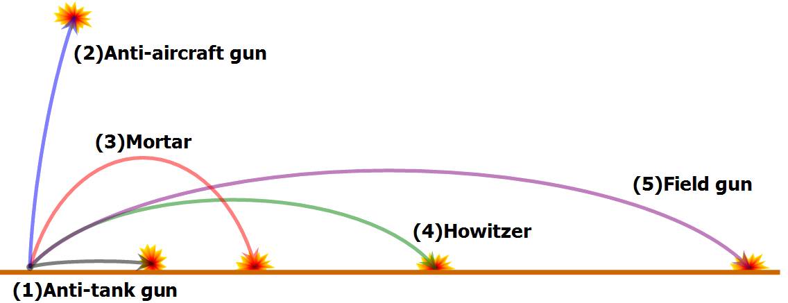
A trajectory can be described mathematically either by the geometry of the path, or as the position of the object over time and requires exact knowledge of both position and velocity.
Heisenberg argued that in the quantum world, trajectories do not exist.
Probabilities take the Place of Trajectories
Experiments show that you will find the electron at some definite location, unlike a wave. But if you set up exactly the same situation and measure it again, you will find the electron in a different location, often far outside any experimental uncertainty in your measurement. Repeated measurements will display a statistical distribution of locations that appears wavelike.
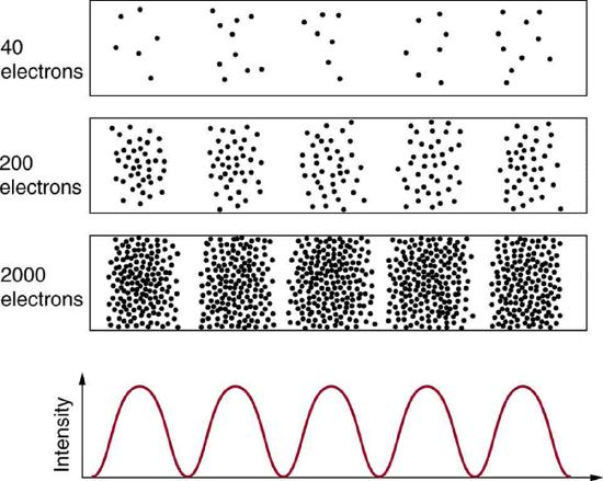
After de Broglie proposed the wave nature of matter, many physicists, including Schrödinger and Heisenberg, explored the consequences. The idea quickly emerged that, because of its wave character, a particle’s trajectory and destination cannot be precisely predicted for each particle individually. However, each particle goes to a definite place. After compiling enough data, you get a distribution related to the particle’s wavelength and diffraction pattern. There is a certain probability of finding the particle at a given location, and the overall pattern is called a probability distribution.
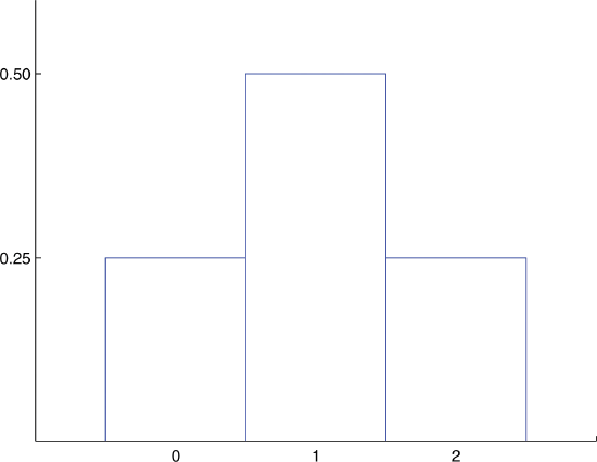
Build the probability distributions for flipping two coins.
- Answer:
-
-
Probability Distribution for Tossing a Fair Coin Twice
What about two dice?
- Answer
-
We will make a table of the probabilities for the sum of the dice. The possibilities are: 2,3,4,5,6,7,8,9,10,11,12.
Probability Distribution Table \(x\) 2 3 4 5 6 7 8 9 10 11 12 \(P(x)\) 1/36 2/36 3/36 4/36 5/36 6/36 5/36 4/36 3/36 2/36 1/36 -
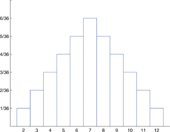
Probability Distribution for Tossing Two Fair Dice. This is a discrete (i.e., quantized) probability distributions, not continuous.
The probability distributions above have several properties of interest:
- The integrated value (\(A\)) MUST be 1: This is the sum over the distribution over all possible values of \(x\). Graphically, this is the area under the distribution. \[ A= \int_{-\infty}^{\infty} D(x)\, dx = 1 \label{1}\]
- The expectation value (\(\langle x \rangle \)): This is a different term that is used synonymously with the average (or mean) of \(x\) over the distribution. The mean is given by \[ \bar{x} = \langle x \rangle = \int_{a}^{b} x D(x)\, dx \label{3}\]
- The most probable value (\(x_{mp}\)): This is the value of \(x\) at the peak of \(D(x)\). This is determined from basic calculus for determining extrema and via identifying when the derivative of the distribution is zero. \[ \left( \dfrac{dD(x)}{dx} \right)_{x_{mp}} = 0 \label{4}\]
- The standard deviation (\(\sigma_x\)): This is the a measure of the spread of the distribution and is given by \[ \sigma_x^2 = \int_{a}^{b} (x-\bar{x})^2 D(x) \,dx \label{5}\]
Heisenberg Uncertainly Principle
It is mathematically possible to express the uncertainty that, Heisenberg concluded, always exists if one attempts to measure the momentum and position of particles. First, we must define the variable “\(x\)” as the position of the particle, and define “\(p\)” as the momentum of the particle. The momentum of a photon of light is known to simply be its frequency, expressed by the ratio \(h/λ\), where h represents Planck’s constant and \(λ\) represents the wavelength of the photon.
\[\Delta{p}\Delta{x} \ge \dfrac{h}{4\pi} \label{1.9.5}\]
What this equation reveals is that the more accurately a particle’s position is known, or the smaller \(Δx\) is, the less accurately the momentum of the particle \(Δp\) is known. Mathematically, this occurs because the smaller \(Δx\) becomes, the larger \(Δ\)p must become in order to satisfy the inequality. However, the more accurately momentum is known the less accurately position is known.
with \(\hbar = \frac{h}{2\pi}= 1.0545718 \times 10^{-34}\; m^2 \cdot kg / s\).
The uncertainty principle is inherent in the properties of all wave-like systems, and that it arises in quantum mechanics simply due to the matter wave nature of all quantum objects.
Equation \(\ref{1.9.5}\) reveals that the more accurately a particle’s position is known (the smaller \(Δx\) is), the less accurately the momentum of the particle in the x direction (\(Δp_x\)) is known. Mathematically, this occurs because the smaller \(Δx\) becomes, the larger \(Δp_x\) must become in order to satisfy the inequality. However, the more accurately momentum is known the less accurately position is known (Figure \(\PageIndex{1}\)).
Determine the minimum uncertainties in the positions of the following objects if their speeds are known with a precision of \(1.0 \times 10^{-3} m/s\):
- an electron and
- a bowling ball of mass 6.0 kg.
- Strategy:
-
Given the uncertainty in speed \(\Delta v = 1.0 \times 10^{-3} m/s\), we have to first determine the uncertainty in momentum \(\Delta p = m\Delta v\) and then find the uncertainty in position \(\Delta x = \hbar /(2\Delta p)\).
- Answer 1 For the electron:
-
For the electron
\[\Delta p = m\Delta v = (9.1 \times 10^{-31} kg)(1.0 \times 10^{-3}m/s) = 9.1 \times 10^{-34} kg \cdot m/s,\nonumber\]
\[\Delta x = \frac{\hbar}{2\Delta p} = 5.8 \space cm. \nonumber\]
- Answer 2 For the bowling ball:
-
For the bowling ball
\[\Delta p = m\Delta v = (6.0 \space kg)(1.0 \times 10^{-3}m/s) = 6.0 \times 10^{-3} kg \cdot m/s, \nonumber\]
\[\Delta x = \frac{\hbar}{2\Delta p} = 8.8 \times 10^{-33}m. \nonumber\]
- Significance
-
Unlike the position uncertainty for the electron, the position uncertainty for the bowling ball is immeasurably small. Planck’s constant is very small, so the limitations imposed by the uncertainty principle are not noticeable in macroscopic systems such as a bowling ball.
Heisenberg Uncertainly Principle will be discussed later in more details, but is topically responsible for the existence of atoms
- Heisenberg get pulled over for speeding by the police. The officer asks him "Do you know how fast you were going?"
- Heisenberg replies, "No, but we know exactly where we are!"
- The officer looks at him confused and says "you were going 108 miles per hour!"
- Heisenberg throws his arms up and cries, "Great! Now we're lost!"
- Answer
-
Contributors and Attributions
- David M. Harrison, Department of Physics, University of Toronto
- Peter Kelley, Department of Chemistry, University of California, Davis