
Grading on a Curve (Chem 2A - Madsen)
- Page ID
- 19116
\( \newcommand{\vecs}[1]{\overset { \scriptstyle \rightharpoonup} {\mathbf{#1}} } \)
\( \newcommand{\vecd}[1]{\overset{-\!-\!\rightharpoonup}{\vphantom{a}\smash {#1}}} \)
\( \newcommand{\dsum}{\displaystyle\sum\limits} \)
\( \newcommand{\dint}{\displaystyle\int\limits} \)
\( \newcommand{\dlim}{\displaystyle\lim\limits} \)
\( \newcommand{\id}{\mathrm{id}}\) \( \newcommand{\Span}{\mathrm{span}}\)
( \newcommand{\kernel}{\mathrm{null}\,}\) \( \newcommand{\range}{\mathrm{range}\,}\)
\( \newcommand{\RealPart}{\mathrm{Re}}\) \( \newcommand{\ImaginaryPart}{\mathrm{Im}}\)
\( \newcommand{\Argument}{\mathrm{Arg}}\) \( \newcommand{\norm}[1]{\| #1 \|}\)
\( \newcommand{\inner}[2]{\langle #1, #2 \rangle}\)
\( \newcommand{\Span}{\mathrm{span}}\)
\( \newcommand{\id}{\mathrm{id}}\)
\( \newcommand{\Span}{\mathrm{span}}\)
\( \newcommand{\kernel}{\mathrm{null}\,}\)
\( \newcommand{\range}{\mathrm{range}\,}\)
\( \newcommand{\RealPart}{\mathrm{Re}}\)
\( \newcommand{\ImaginaryPart}{\mathrm{Im}}\)
\( \newcommand{\Argument}{\mathrm{Arg}}\)
\( \newcommand{\norm}[1]{\| #1 \|}\)
\( \newcommand{\inner}[2]{\langle #1, #2 \rangle}\)
\( \newcommand{\Span}{\mathrm{span}}\) \( \newcommand{\AA}{\unicode[.8,0]{x212B}}\)
\( \newcommand{\vectorA}[1]{\vec{#1}} % arrow\)
\( \newcommand{\vectorAt}[1]{\vec{\text{#1}}} % arrow\)
\( \newcommand{\vectorB}[1]{\overset { \scriptstyle \rightharpoonup} {\mathbf{#1}} } \)
\( \newcommand{\vectorC}[1]{\textbf{#1}} \)
\( \newcommand{\vectorD}[1]{\overrightarrow{#1}} \)
\( \newcommand{\vectorDt}[1]{\overrightarrow{\text{#1}}} \)
\( \newcommand{\vectE}[1]{\overset{-\!-\!\rightharpoonup}{\vphantom{a}\smash{\mathbf {#1}}}} \)
\( \newcommand{\vecs}[1]{\overset { \scriptstyle \rightharpoonup} {\mathbf{#1}} } \)
\(\newcommand{\longvect}{\overrightarrow}\)
\( \newcommand{\vecd}[1]{\overset{-\!-\!\rightharpoonup}{\vphantom{a}\smash {#1}}} \)
\(\newcommand{\avec}{\mathbf a}\) \(\newcommand{\bvec}{\mathbf b}\) \(\newcommand{\cvec}{\mathbf c}\) \(\newcommand{\dvec}{\mathbf d}\) \(\newcommand{\dtil}{\widetilde{\mathbf d}}\) \(\newcommand{\evec}{\mathbf e}\) \(\newcommand{\fvec}{\mathbf f}\) \(\newcommand{\nvec}{\mathbf n}\) \(\newcommand{\pvec}{\mathbf p}\) \(\newcommand{\qvec}{\mathbf q}\) \(\newcommand{\svec}{\mathbf s}\) \(\newcommand{\tvec}{\mathbf t}\) \(\newcommand{\uvec}{\mathbf u}\) \(\newcommand{\vvec}{\mathbf v}\) \(\newcommand{\wvec}{\mathbf w}\) \(\newcommand{\xvec}{\mathbf x}\) \(\newcommand{\yvec}{\mathbf y}\) \(\newcommand{\zvec}{\mathbf z}\) \(\newcommand{\rvec}{\mathbf r}\) \(\newcommand{\mvec}{\mathbf m}\) \(\newcommand{\zerovec}{\mathbf 0}\) \(\newcommand{\onevec}{\mathbf 1}\) \(\newcommand{\real}{\mathbb R}\) \(\newcommand{\twovec}[2]{\left[\begin{array}{r}#1 \\ #2 \end{array}\right]}\) \(\newcommand{\ctwovec}[2]{\left[\begin{array}{c}#1 \\ #2 \end{array}\right]}\) \(\newcommand{\threevec}[3]{\left[\begin{array}{r}#1 \\ #2 \\ #3 \end{array}\right]}\) \(\newcommand{\cthreevec}[3]{\left[\begin{array}{c}#1 \\ #2 \\ #3 \end{array}\right]}\) \(\newcommand{\fourvec}[4]{\left[\begin{array}{r}#1 \\ #2 \\ #3 \\ #4 \end{array}\right]}\) \(\newcommand{\cfourvec}[4]{\left[\begin{array}{c}#1 \\ #2 \\ #3 \\ #4 \end{array}\right]}\) \(\newcommand{\fivevec}[5]{\left[\begin{array}{r}#1 \\ #2 \\ #3 \\ #4 \\ #5 \\ \end{array}\right]}\) \(\newcommand{\cfivevec}[5]{\left[\begin{array}{c}#1 \\ #2 \\ #3 \\ #4 \\ #5 \\ \end{array}\right]}\) \(\newcommand{\mattwo}[4]{\left[\begin{array}{rr}#1 \amp #2 \\ #3 \amp #4 \\ \end{array}\right]}\) \(\newcommand{\laspan}[1]{\text{Span}\{#1\}}\) \(\newcommand{\bcal}{\cal B}\) \(\newcommand{\ccal}{\cal C}\) \(\newcommand{\scal}{\cal S}\) \(\newcommand{\wcal}{\cal W}\) \(\newcommand{\ecal}{\cal E}\) \(\newcommand{\coords}[2]{\left\{#1\right\}_{#2}}\) \(\newcommand{\gray}[1]{\color{gray}{#1}}\) \(\newcommand{\lgray}[1]{\color{lightgray}{#1}}\) \(\newcommand{\rank}{\operatorname{rank}}\) \(\newcommand{\row}{\text{Row}}\) \(\newcommand{\col}{\text{Col}}\) \(\renewcommand{\row}{\text{Row}}\) \(\newcommand{\nul}{\text{Nul}}\) \(\newcommand{\var}{\text{Var}}\) \(\newcommand{\corr}{\text{corr}}\) \(\newcommand{\len}[1]{\left|#1\right|}\) \(\newcommand{\bbar}{\overline{\bvec}}\) \(\newcommand{\bhat}{\widehat{\bvec}}\) \(\newcommand{\bperp}{\bvec^\perp}\) \(\newcommand{\xhat}{\widehat{\xvec}}\) \(\newcommand{\vhat}{\widehat{\vvec}}\) \(\newcommand{\uhat}{\widehat{\uvec}}\) \(\newcommand{\what}{\widehat{\wvec}}\) \(\newcommand{\Sighat}{\widehat{\Sigma}}\) \(\newcommand{\lt}{<}\) \(\newcommand{\gt}{>}\) \(\newcommand{\amp}{&}\) \(\definecolor{fillinmathshade}{gray}{0.9}\)| UC Davis CHE 2A: General Chemistry | Reading Assignments Homework Problems Homework Solutions Grading on a Curve | |
| Unit I: Atomic Theory Unit II: Chemical Reactions Unit III: Gases Unit IV: Quantum Theory | ||
In education, grading on a curve is a statistical method of assigning grades designed to yield a pre-determined distribution of grades among the students in a class. The term "curve" refers to the "bell curve," the graphical representation of the probability density of the normal distribution (also called the Gaussian distribution).
The Process
The method of applying a curve in Chem 2A (Fall Quarter 2010) uses these three steps:
- First, numeric scores are assigned to the students.
- The scores for all exams and labs are added up relative to the weight they are given in the Syllabus
25% midterm1 + 25% midterm2 + 40% final + 10% lab
- Grades are assigned depending on the average and standard deviation of the distribution of the added scores for all students.
Constructing the Curve via Deviations From Mean)
The "curve" or grading distribution is based on how far the final score is from the average of the whole class in terms of standard deviations.
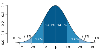
The mean will be the cutoff C/C+ (same grade for all sections of the class). One standard deviation above that will be the cutoff between a B/B+, two standard deviations will be an A/A+. To estimate your own grade you first have to calculate where your score is relative to the overall class:
\[S = \dfrac{(\rm your~score)-(\rm average)}{\rm stdev}\]
Then you can estimate your grade according to the table:
| Grade | S | Grade | S |
|---|---|---|---|
| A+ | 2 and above | C | -1/3 to 0 |
| A | +5/3 to +2 | C- | -2/3 to -1/3 |
| A- | +4/3 to +5/3 | D+ | -1 to -2/3 |
| B+ | +1 to +4/3 | D | -4/3 to -1 |
| B | +2/3 to +1 | D- | -5/3 to -4/3 |
| B- | +1/3 to +2/3 | F | below -5/3 |
| C+ | 0 to +1/3 |
| Example |
|---|
|
What Matters is the Score Relative to Others
Since curving is designed to normalize the class to a known average, the absolute grade for a specific student is not the relevant measure of performance. The proper measure is the deviation from the mean (in factors of standard deviation).
For example: Student A in class #1 may get a 90% on the final score, whereas student B in class #2 may get a 85% Which student gets the higher grade for the class?
- On an absolute grading scale, one would presume student A would get the higher grade, however a grade based on a curve requires more enough information to answer.
- If the mean for class #1 is 84% and the mean for class #2 is 70%, then student B has a greater deviation from the respective mean of the class (85%-70%=15%) vs. (90%-84%=6%) for student A.
- This is still not enough, since it is necessary to ask how great of a spread of scores around the mean is the distribution. This is quantified via a standard deviation. Hence, if the standard deviation of the scores in class #1 is 6% and for class #2 it is 20%, then student A is 1.0 standard deviations above the mean and student B is 15/20=0.75 standard deviations above the mean. The answer to which student gets the higher grade is student A since he/she is a greater number of deviations above the mean. This is the only meaningful measure for a student's performance with a mean.
The Importance of having a score distribution centered around 50%
Believe it or not, the best grade distribution is centered around 50%. That is, the class mean is in the middle of possible range of scores, which provides students the full range of opportunity to excel (by having a greater deviation from the mean). Distributions with higher averages (e.g. 75% to 80%) may initially appear great to the student (mostly by boosting egos), but really limit the students abilities to perform well. For example, if a class had a final average of 80%, and a standard deviation of 15%, then the BEST any student can do (100% absolute score) is to get 20/15= 1.33 x standard deviation above the mean. As shown below, that can mean a potential maximum of a A- for the class. This is a greatly undesired result and does a grave disservice to advance students.
FAQ: I got a "X" on the test, what do I need to get an overall grade "Y"?
Many students ask me if it is possible for them to still pass the class/get an A/fill in the blank if they got a certain score on the first midterm. Using the formalism described above you can calculate this for yourself. First calculate your score in terms of number of standard deviations from the mean (S) as described above. For the overall class you can now calculate your grade using the weights for each exam:
\[S_{\rm class} = 0.25 S_1 + 0.25 S_2 + 0.4 S_f + 0.1S_{\rm lab} \]
Please note that the average for the lab is usually very high and the standard deviation is very narrow. Therefore, do NOT count on your lab to improve your score. It can drag you down if it is low, but it doesn't help you much if it is high. Scoring a perfect 100% on your labs will only count as a 1 in the overall formula.
| Example |
|---|
| Student gets 38 points on an exam that has an average of 59 points and a standard deviation of 21, so one standard deviation below the mean. Can he/she still pass? Solution \[S_{\rm class} = 0.25 \times (-1) + 0.25 S_2 + 0.4 S_f + 0.1 \times (0) > -2/3 \] You can play around with numbers on the other two exams to see what is necessary, but it is definitely still possible to pass the class with a score of 38 points on the first exam |