10.9 Essential Skills 5
- Page ID
- 19114
\( \newcommand{\vecs}[1]{\overset { \scriptstyle \rightharpoonup} {\mathbf{#1}} } \)
\( \newcommand{\vecd}[1]{\overset{-\!-\!\rightharpoonup}{\vphantom{a}\smash {#1}}} \)
\( \newcommand{\id}{\mathrm{id}}\) \( \newcommand{\Span}{\mathrm{span}}\)
( \newcommand{\kernel}{\mathrm{null}\,}\) \( \newcommand{\range}{\mathrm{range}\,}\)
\( \newcommand{\RealPart}{\mathrm{Re}}\) \( \newcommand{\ImaginaryPart}{\mathrm{Im}}\)
\( \newcommand{\Argument}{\mathrm{Arg}}\) \( \newcommand{\norm}[1]{\| #1 \|}\)
\( \newcommand{\inner}[2]{\langle #1, #2 \rangle}\)
\( \newcommand{\Span}{\mathrm{span}}\)
\( \newcommand{\id}{\mathrm{id}}\)
\( \newcommand{\Span}{\mathrm{span}}\)
\( \newcommand{\kernel}{\mathrm{null}\,}\)
\( \newcommand{\range}{\mathrm{range}\,}\)
\( \newcommand{\RealPart}{\mathrm{Re}}\)
\( \newcommand{\ImaginaryPart}{\mathrm{Im}}\)
\( \newcommand{\Argument}{\mathrm{Arg}}\)
\( \newcommand{\norm}[1]{\| #1 \|}\)
\( \newcommand{\inner}[2]{\langle #1, #2 \rangle}\)
\( \newcommand{\Span}{\mathrm{span}}\) \( \newcommand{\AA}{\unicode[.8,0]{x212B}}\)
\( \newcommand{\vectorA}[1]{\vec{#1}} % arrow\)
\( \newcommand{\vectorAt}[1]{\vec{\text{#1}}} % arrow\)
\( \newcommand{\vectorB}[1]{\overset { \scriptstyle \rightharpoonup} {\mathbf{#1}} } \)
\( \newcommand{\vectorC}[1]{\textbf{#1}} \)
\( \newcommand{\vectorD}[1]{\overrightarrow{#1}} \)
\( \newcommand{\vectorDt}[1]{\overrightarrow{\text{#1}}} \)
\( \newcommand{\vectE}[1]{\overset{-\!-\!\rightharpoonup}{\vphantom{a}\smash{\mathbf {#1}}}} \)
\( \newcommand{\vecs}[1]{\overset { \scriptstyle \rightharpoonup} {\mathbf{#1}} } \)
\( \newcommand{\vecd}[1]{\overset{-\!-\!\rightharpoonup}{\vphantom{a}\smash {#1}}} \)
\(\newcommand{\avec}{\mathbf a}\) \(\newcommand{\bvec}{\mathbf b}\) \(\newcommand{\cvec}{\mathbf c}\) \(\newcommand{\dvec}{\mathbf d}\) \(\newcommand{\dtil}{\widetilde{\mathbf d}}\) \(\newcommand{\evec}{\mathbf e}\) \(\newcommand{\fvec}{\mathbf f}\) \(\newcommand{\nvec}{\mathbf n}\) \(\newcommand{\pvec}{\mathbf p}\) \(\newcommand{\qvec}{\mathbf q}\) \(\newcommand{\svec}{\mathbf s}\) \(\newcommand{\tvec}{\mathbf t}\) \(\newcommand{\uvec}{\mathbf u}\) \(\newcommand{\vvec}{\mathbf v}\) \(\newcommand{\wvec}{\mathbf w}\) \(\newcommand{\xvec}{\mathbf x}\) \(\newcommand{\yvec}{\mathbf y}\) \(\newcommand{\zvec}{\mathbf z}\) \(\newcommand{\rvec}{\mathbf r}\) \(\newcommand{\mvec}{\mathbf m}\) \(\newcommand{\zerovec}{\mathbf 0}\) \(\newcommand{\onevec}{\mathbf 1}\) \(\newcommand{\real}{\mathbb R}\) \(\newcommand{\twovec}[2]{\left[\begin{array}{r}#1 \\ #2 \end{array}\right]}\) \(\newcommand{\ctwovec}[2]{\left[\begin{array}{c}#1 \\ #2 \end{array}\right]}\) \(\newcommand{\threevec}[3]{\left[\begin{array}{r}#1 \\ #2 \\ #3 \end{array}\right]}\) \(\newcommand{\cthreevec}[3]{\left[\begin{array}{c}#1 \\ #2 \\ #3 \end{array}\right]}\) \(\newcommand{\fourvec}[4]{\left[\begin{array}{r}#1 \\ #2 \\ #3 \\ #4 \end{array}\right]}\) \(\newcommand{\cfourvec}[4]{\left[\begin{array}{c}#1 \\ #2 \\ #3 \\ #4 \end{array}\right]}\) \(\newcommand{\fivevec}[5]{\left[\begin{array}{r}#1 \\ #2 \\ #3 \\ #4 \\ #5 \\ \end{array}\right]}\) \(\newcommand{\cfivevec}[5]{\left[\begin{array}{c}#1 \\ #2 \\ #3 \\ #4 \\ #5 \\ \end{array}\right]}\) \(\newcommand{\mattwo}[4]{\left[\begin{array}{rr}#1 \amp #2 \\ #3 \amp #4 \\ \end{array}\right]}\) \(\newcommand{\laspan}[1]{\text{Span}\{#1\}}\) \(\newcommand{\bcal}{\cal B}\) \(\newcommand{\ccal}{\cal C}\) \(\newcommand{\scal}{\cal S}\) \(\newcommand{\wcal}{\cal W}\) \(\newcommand{\ecal}{\cal E}\) \(\newcommand{\coords}[2]{\left\{#1\right\}_{#2}}\) \(\newcommand{\gray}[1]{\color{gray}{#1}}\) \(\newcommand{\lgray}[1]{\color{lightgray}{#1}}\) \(\newcommand{\rank}{\operatorname{rank}}\) \(\newcommand{\row}{\text{Row}}\) \(\newcommand{\col}{\text{Col}}\) \(\renewcommand{\row}{\text{Row}}\) \(\newcommand{\nul}{\text{Nul}}\) \(\newcommand{\var}{\text{Var}}\) \(\newcommand{\corr}{\text{corr}}\) \(\newcommand{\len}[1]{\left|#1\right|}\) \(\newcommand{\bbar}{\overline{\bvec}}\) \(\newcommand{\bhat}{\widehat{\bvec}}\) \(\newcommand{\bperp}{\bvec^\perp}\) \(\newcommand{\xhat}{\widehat{\xvec}}\) \(\newcommand{\vhat}{\widehat{\vvec}}\) \(\newcommand{\uhat}{\widehat{\uvec}}\) \(\newcommand{\what}{\widehat{\wvec}}\) \(\newcommand{\Sighat}{\widehat{\Sigma}}\) \(\newcommand{\lt}{<}\) \(\newcommand{\gt}{>}\) \(\newcommand{\amp}{&}\) \(\definecolor{fillinmathshade}{gray}{0.9}\)The topics of ths Module are to
- Preparing a Graph
- Interpreting a Graph
Previous Essential Skills sections presented the fundamental mathematical operations you need to know to solve problems by manipulating chemical equations. This section describes how to prepare and interpret graphs, two additional skills that chemistry students must have to understand concepts and solve problems.
Preparing a Graph
A graph is a pictorial representation of a mathematical relationship. It is an extremely effective tool for understanding and communicating the relationship between two or more variables. Each axis is labeled with the name of the variable to which it corresponds, along with the unit in which the variable is measured, and each axis is divided by tic marks or grid lines into segments that represent those units (or multiples). The scale of the divisions should be chosen so that the plotted points are distributed across the entire graph. Whenever possible, data points should be combined with a bar that intersects the data point and indicates the range of error of the measurement, although for simplicity the bars are frequently omitted in undergraduate textbooks. Lines or curves that represent theoretical or computational results are drawn using a “best-fit” approach; that is, data points are not connected as a series of straight-line segments; rather, a smooth line or curve is drawn that provides the best fit to the plotted data.
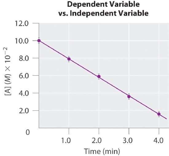
The independent variable is usually assigned to the horizontal, or x, axis (also called the abscissa), and the dependent variable to the vertical, or y, axis (called the ordinate). Let’s examine, for example, an experiment in which we are interested in plotting the change in the concentration of compound A with time. Because time does not depend on the concentration of A but the concentration of A does depend on the amount of time that has passed during the reaction, time is the independent variable and concentration is the dependent variable. In this case, the time is assigned to the horizontal axis and the concentration of A to the vertical axis.
We may plot more than one dependent variable on a graph, but the lines or curves corresponding to each set of data must be clearly identified with labels, different types of lines (a dashed line, for example), or different symbols for the respective data points (e.g., a triangle versus a circle). When words are used to label a line or curve, either a key identifying the different sets of data or a label placed next to each line or curve is used.
Interpreting a Graph
Two types of graphs are frequently encountered in beginning chemistry courses: linear and log-linear. Here we describe each type.
Linear Graphs
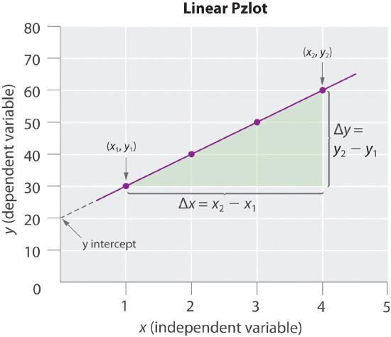
In a linear graph, the plot of the relationship between the variables is a straight line and thus can be expressed by the equation for a straight line:
\[y = mx + b\]
where \(m\) is the slope of the line and \(b\) is the point where the line intersects the vertical axis (where \(x = 0\)), called the y-intercept. The slope is calculated using the following formula:
For accuracy, two widely separated points should be selected for use in the formula to minimize the effects of any reporting or measurement errors that may have occurred in any given region of the graph. For example, when concentrations are measured, limitations in the sensitivity of an instrument as well as human error may result in measurements being less accurate for samples with low concentrations than for those that are more concentrated. The graph of the change in the concentration of A with time is an example of a linear graph. The key features of a linear plot are shown on the generic example.
It is important to remember that when a graphical procedure is used to calculate a slope, the scale on each axis must be of the same order (they must have the same exponent). For example, although acceleration is a change in velocity over time (Δv/Δt), the slope of a linear plot of velocity versus time only gives the correct value for acceleration (m/s2) if the average acceleration over the interval and the instantaneous acceleration are identical; that is, the acceleration must be constant over the same interval.
Log-Linear Graphs
A log-linear plot is a representation of the following general mathematical relationship:
\[y = Ac^{mx}\]
Here, y is equal to some value \(Ac\) when \(x = 0\). Taking the logarithm of both sides produces
\[\log y = \log A + mx \log c = (m \log c)x + \log A\]
When expressed in this form, the equation is that of a straight line (y = mx + b), where the plot of y is on a logarithmic axis and (m log c)x is on a linear axis. This type of graph is known as a log-linear plot. Log-linear plots are particularly useful for graphing changes in pH versus changes in the concentration of another substance. One example of a log-linear plot, where \(y = [HA]\) and \(x = pH\), is shown here:
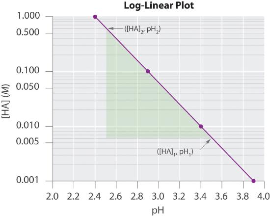
Using any point along the line (e.g., [HA] = 0.100, pH = 2.9), we can then calculate the y-intercept (pH = 0):
Thus at a pH of 0.0, log[HA] = 4.8 and [HA] = 6.31 × 10⁴ M. The exercises provide practice in drawing and interpreting graphs.
Skill Builder ES1
-
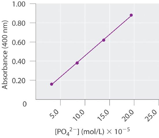
The absorbance of light by various aqueous solutions of phosphate was measured and tabulated as follows:
Absorbance (400 nm) PO43− (mol/L) 0.16 3.2 × 10⁻⁵ 0.38 8.4 × 10⁻⁵ 0.62 13.8 × 10⁻⁵ 0.88 19.4 × 10⁻⁵ Graph the data with the dependent variable on the y axis and the independent variable on the x axis and then calculate the slope. If a sample has an absorbance of 0.45, what is the phosphate concentration in the sample?
-
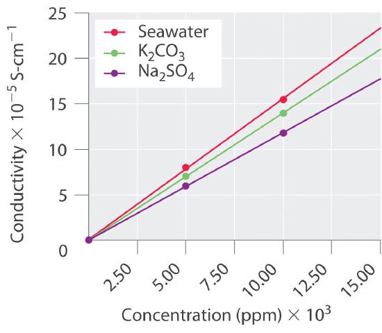
The following table lists the conductivity of three aqueous solutions with varying concentrations. Create a plot from these data and then predict the conductivity of each sample at a concentration of 15.0 × 10³ ppm.
0 ppm 5.00 × 10³ ppm 10.00 × 10³ ppm K2CO3 0.0 7.0 14.0 Seawater 0.0 8.0 15.5 Na2SO4 0.0 6.0 11.8
Solution:
-
Absorbance is the dependent variable, and concentration is the independent variable. We calculate the slope using two widely separated data points:
According to our graph, the y-intercept, b, is 0.00. Thus when y = 0.45,
0.45 = (4.3 × 10³)(x) + 0.00 x = 10 × 10−5This is in good agreement with a graphical determination of the phosphate concentration at an absorbance of 0.45, which gives a value of 10.2 × 10⁻⁵ mol/L.
-
Conductivity is the dependent variable, and concentration is the independent variable. From our graph, at 15.0 × 10³ ppm, the conductivity of K2CO3 is predicted to be 21; that of seawater, 24; and that of Na2SO4, 18.