5.10: Fourier Transform (pulsed) NMR - The way things are really done these days
- Page ID
- 369989
\( \newcommand{\vecs}[1]{\overset { \scriptstyle \rightharpoonup} {\mathbf{#1}} } \)
\( \newcommand{\vecd}[1]{\overset{-\!-\!\rightharpoonup}{\vphantom{a}\smash {#1}}} \)
\( \newcommand{\id}{\mathrm{id}}\) \( \newcommand{\Span}{\mathrm{span}}\)
( \newcommand{\kernel}{\mathrm{null}\,}\) \( \newcommand{\range}{\mathrm{range}\,}\)
\( \newcommand{\RealPart}{\mathrm{Re}}\) \( \newcommand{\ImaginaryPart}{\mathrm{Im}}\)
\( \newcommand{\Argument}{\mathrm{Arg}}\) \( \newcommand{\norm}[1]{\| #1 \|}\)
\( \newcommand{\inner}[2]{\langle #1, #2 \rangle}\)
\( \newcommand{\Span}{\mathrm{span}}\)
\( \newcommand{\id}{\mathrm{id}}\)
\( \newcommand{\Span}{\mathrm{span}}\)
\( \newcommand{\kernel}{\mathrm{null}\,}\)
\( \newcommand{\range}{\mathrm{range}\,}\)
\( \newcommand{\RealPart}{\mathrm{Re}}\)
\( \newcommand{\ImaginaryPart}{\mathrm{Im}}\)
\( \newcommand{\Argument}{\mathrm{Arg}}\)
\( \newcommand{\norm}[1]{\| #1 \|}\)
\( \newcommand{\inner}[2]{\langle #1, #2 \rangle}\)
\( \newcommand{\Span}{\mathrm{span}}\) \( \newcommand{\AA}{\unicode[.8,0]{x212B}}\)
\( \newcommand{\vectorA}[1]{\vec{#1}} % arrow\)
\( \newcommand{\vectorAt}[1]{\vec{\text{#1}}} % arrow\)
\( \newcommand{\vectorB}[1]{\overset { \scriptstyle \rightharpoonup} {\mathbf{#1}} } \)
\( \newcommand{\vectorC}[1]{\textbf{#1}} \)
\( \newcommand{\vectorD}[1]{\overrightarrow{#1}} \)
\( \newcommand{\vectorDt}[1]{\overrightarrow{\text{#1}}} \)
\( \newcommand{\vectE}[1]{\overset{-\!-\!\rightharpoonup}{\vphantom{a}\smash{\mathbf {#1}}}} \)
\( \newcommand{\vecs}[1]{\overset { \scriptstyle \rightharpoonup} {\mathbf{#1}} } \)
\( \newcommand{\vecd}[1]{\overset{-\!-\!\rightharpoonup}{\vphantom{a}\smash {#1}}} \)
\(\newcommand{\avec}{\mathbf a}\) \(\newcommand{\bvec}{\mathbf b}\) \(\newcommand{\cvec}{\mathbf c}\) \(\newcommand{\dvec}{\mathbf d}\) \(\newcommand{\dtil}{\widetilde{\mathbf d}}\) \(\newcommand{\evec}{\mathbf e}\) \(\newcommand{\fvec}{\mathbf f}\) \(\newcommand{\nvec}{\mathbf n}\) \(\newcommand{\pvec}{\mathbf p}\) \(\newcommand{\qvec}{\mathbf q}\) \(\newcommand{\svec}{\mathbf s}\) \(\newcommand{\tvec}{\mathbf t}\) \(\newcommand{\uvec}{\mathbf u}\) \(\newcommand{\vvec}{\mathbf v}\) \(\newcommand{\wvec}{\mathbf w}\) \(\newcommand{\xvec}{\mathbf x}\) \(\newcommand{\yvec}{\mathbf y}\) \(\newcommand{\zvec}{\mathbf z}\) \(\newcommand{\rvec}{\mathbf r}\) \(\newcommand{\mvec}{\mathbf m}\) \(\newcommand{\zerovec}{\mathbf 0}\) \(\newcommand{\onevec}{\mathbf 1}\) \(\newcommand{\real}{\mathbb R}\) \(\newcommand{\twovec}[2]{\left[\begin{array}{r}#1 \\ #2 \end{array}\right]}\) \(\newcommand{\ctwovec}[2]{\left[\begin{array}{c}#1 \\ #2 \end{array}\right]}\) \(\newcommand{\threevec}[3]{\left[\begin{array}{r}#1 \\ #2 \\ #3 \end{array}\right]}\) \(\newcommand{\cthreevec}[3]{\left[\begin{array}{c}#1 \\ #2 \\ #3 \end{array}\right]}\) \(\newcommand{\fourvec}[4]{\left[\begin{array}{r}#1 \\ #2 \\ #3 \\ #4 \end{array}\right]}\) \(\newcommand{\cfourvec}[4]{\left[\begin{array}{c}#1 \\ #2 \\ #3 \\ #4 \end{array}\right]}\) \(\newcommand{\fivevec}[5]{\left[\begin{array}{r}#1 \\ #2 \\ #3 \\ #4 \\ #5 \\ \end{array}\right]}\) \(\newcommand{\cfivevec}[5]{\left[\begin{array}{c}#1 \\ #2 \\ #3 \\ #4 \\ #5 \\ \end{array}\right]}\) \(\newcommand{\mattwo}[4]{\left[\begin{array}{rr}#1 \amp #2 \\ #3 \amp #4 \\ \end{array}\right]}\) \(\newcommand{\laspan}[1]{\text{Span}\{#1\}}\) \(\newcommand{\bcal}{\cal B}\) \(\newcommand{\ccal}{\cal C}\) \(\newcommand{\scal}{\cal S}\) \(\newcommand{\wcal}{\cal W}\) \(\newcommand{\ecal}{\cal E}\) \(\newcommand{\coords}[2]{\left\{#1\right\}_{#2}}\) \(\newcommand{\gray}[1]{\color{gray}{#1}}\) \(\newcommand{\lgray}[1]{\color{lightgray}{#1}}\) \(\newcommand{\rank}{\operatorname{rank}}\) \(\newcommand{\row}{\text{Row}}\) \(\newcommand{\col}{\text{Col}}\) \(\renewcommand{\row}{\text{Row}}\) \(\newcommand{\nul}{\text{Nul}}\) \(\newcommand{\var}{\text{Var}}\) \(\newcommand{\corr}{\text{corr}}\) \(\newcommand{\len}[1]{\left|#1\right|}\) \(\newcommand{\bbar}{\overline{\bvec}}\) \(\newcommand{\bhat}{\widehat{\bvec}}\) \(\newcommand{\bperp}{\bvec^\perp}\) \(\newcommand{\xhat}{\widehat{\xvec}}\) \(\newcommand{\vhat}{\widehat{\vvec}}\) \(\newcommand{\uhat}{\widehat{\uvec}}\) \(\newcommand{\what}{\widehat{\wvec}}\) \(\newcommand{\Sighat}{\widehat{\Sigma}}\) \(\newcommand{\lt}{<}\) \(\newcommand{\gt}{>}\) \(\newcommand{\amp}{&}\) \(\definecolor{fillinmathshade}{gray}{0.9}\)Most applications of NMR involve full NMR spectra, that is, the intensity of the NMR signal as a function of frequency. Early attempts to acquire the NMR spectrum more efficiently than simple CW methods involved irradiating simultaneously with more than one frequency. A revolution in NMR occurred when short pulses of radio-frequency were used (centered at the middle of the NMR spectrum). In simple terms, a short square pulse of a given "carrier" frequency "contains" a range of frequencies centered about the carrier frequency, with the range of excitation (bandwidth) being inversely proportional to the pulse duration (the Fourier transform (FT) of an approximate square wave contains contributions from all the frequencies in the neighborhood of the principal frequency). The restricted range of the NMR frequencies made it relatively easy to use short (millisecond to microsecond) RF pulses to excite the entire NMR spectrum.
Applying such a pulse to a set of nuclear spins simultaneously excites all the single-quantum NMR transitions. In terms of the net magnetization vector, this corresponds to tilting the magnetization vector away from its equilibrium position (aligned along the external magnetic field). The out-of-equilibrium magnetization vector precesses about the external magnetic field vector at the NMR frequency of the spins. This oscillating magnetization vector induces a current in a nearby pickup coil, creating an electrical signal oscillating at the NMR frequency. This signal is known as the free induction decay (FID) and contains the vector-sum of the NMR responses from all the excited spins. In order to obtain the frequency-domain NMR spectrum (NMR absorption intensity vs. NMR frequency) this time-domain signal (intensity vs. time) must be FTed. Fortunately the development of FT NMR coincided with the development of digital computers and Fast Fourier Transform algorithms.
An NMR sample may contain many different magnetization components, each with its own Larmor frequency. These magnetization components are associated with the nuclear spin configurations joined by an allowed transition line in the energy level diagram. Based on the number of allowed absorptions due to chemical shifts and spin-spin couplings of the different nuclei in a molecule, an NMR spectrum may contain many different frequency lines.
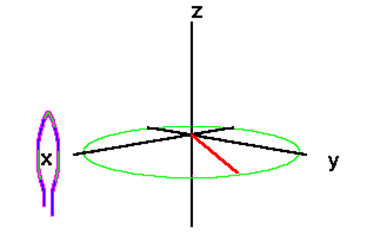
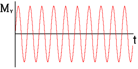
In pulsed NMR spectroscopy, signal is detected after these magnetization vectors are rotated into the XY plane. Once a magnetization vector is in the XY plane it rotates about the direction of the Bo field, the +Z axis. As transverse magnetization rotates about the Z axis, it will induce a current in a coil of wire located around the X axis.
Plotting current as a function of time gives a sine wave.
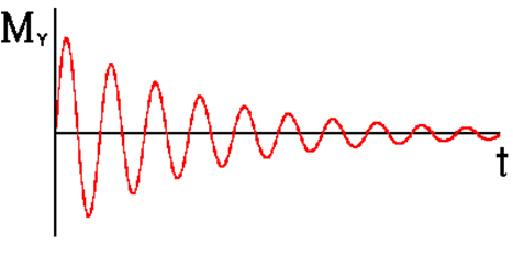
This wave will, of course, decay with time constant \(T_2^{*}\) due to dephasing of the spin packets. This signal is called a free induction decay (FID).
Imagine that \(\vec{H}_{1}\) is turned on @ t=0 exact at a resonance, so that \(\mathrm{H}_{\mathrm{eff}} \sim \vec{H}_{1}\left(\omega_{1}=\omega_{0}\right)\). \(\vec{M}\) will process about \(\vec{H}_1\) (along the u-axis) and after a 90-degree procession, it will lie along the \(v\). At this point, \(\vec{H}_{1}\) is turned off and begin with the entire equilibrium magnetization \(M_o\) along the v-axis. This called a 90 pulse, because the \(\vec{H}_1\) field is pulsed long enough for \(M\) to process 90 degrees about \(\vec{H}_1\).
\[\theta=\gamma H_{1} t_{p} \nonumber \]
where \(t_p\) is the time duration of the pulse. If \(\vec{H}_{1}\) is large enough \(t_p \ll T_2\) so (transverse) relaxation during the pulse can be ignore.
A \(\theta=90^{\circ}\) Pulse
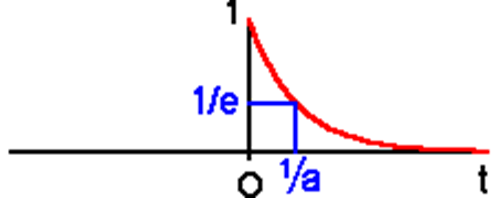
\(M_{v}(0) = M_{0}\), but this will decay with \(T_2\):
\[M_{v}(t)=M_{0} \exp \left(-t / T_{2}\right) \nonumber \]
in the rotating frame….
A coil setup to pick p the signals will observed a decaying cosine signal
\[M_{\perp}(t)=M_{0} \exp \left(-t / T_{2}\right) \cos (\omega t) \nonumber \]
with \(\omega \approx \omega_{\circ}\), since not all process at exactly \(\omega_{\circ}\) because of line width or inhomogeneity).
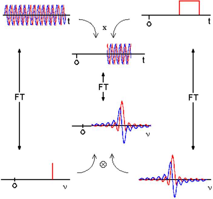
We have a non-periodic \(x(t)\) that can be Fourier Transformed. We know that it is a single function of cosine and exponential decay, the Fourier Transform (in frequency space) will be a convolution of the Fourier Transforms of \(\cos(\omega t)\) and the exponential decay. The factor is analogous to a rectangular window function which produces a \(sinc(x)\) function: \(\sin(x)/x\) centered at \(\pm \omega\). What do we expect for the whole function? A Fourier Transform of \(\exp \left(-t / T_{2}\right)\) centered at \(\pm \omega\).
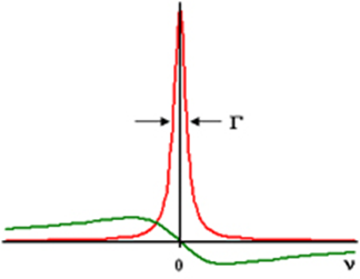
\(M_{\perp}(t)\) is neither symmetric or antisymmetric about \(t=0\), thus we expect non-zero real and imaginary components of \(X(\omega)\), the FT of \(M_{1}(t)\).
\[X(\omega)=A(\omega)+i D(\omega) \nonumber \]
where \(A\) and \(D\) are the real and imaginary part of the Fourier Transform. Here \(A(\omega)\) is the absorption and \(D(\omega)\) is the dispersive components to the signal.
The upshot for FT NMR
Fourier Transform NMR is an example of a set of damped oscillators (nuclei) that have individual resonance frequencies. Each frequency is characterized by its own \(\tau_2\); this damping time constant is called \(T_2\). Thus each resonance contributes to the total FT a set of signals analogous to those represented above for a single damped oscillator. All oscillators are excited simultaneously by a broadband radio-frequency pulse. The decaying oscillators are sampled and Fourier Analyzed.
The \(\vec{H}_1\) field is applied at \(f_0\) (approximately the Larmour Frequency of all protons in sample). The RF is windows through a rectangular window of length \(t_p\).
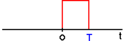
The spectral content is given by the \(\text{sinc} x\) function center \(\pm f_0\): (sin(2 t))/(2 t) with imaginary component: -(sin2(2 t))/( t)
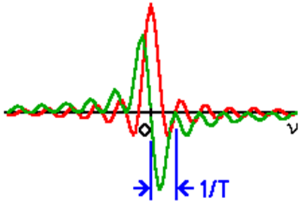
All protons with in a bandwidth of \(\sim \Delta f_{p}=\frac{2}{t_{p}}\) about \(f_0\) will be tipped away from z toward the v plane and will contribute their own frequencies to the FID. So, if we want \(\Delta f_{p}\) to be ~2,000 Hz to cover a large range of chemical shifts, we need a \(t_p\) of 10-3 s.
\[\Delta f_{p}=\frac{2}{t_{p}}=2000 \mathrm{~Hz} \nonumber \]
so \(t_{p}=10^{-3} s\).
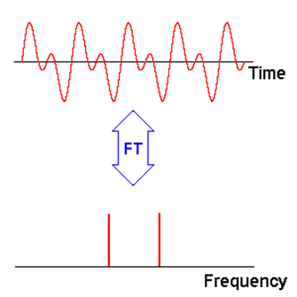
The convolution theorem says that the FT of a convolution of two functions is proportional to the products of the individual Fourier transforms, and vice versa.
If \(f(\omega) = FT(f(t))\) and \(g(\omega) = FT( g(t) )\) then \(f(\omega) g(\omega ) = FT( g(t) f(t) )\) and \(f\omega) \times g(\omega) = FT( g(t) f(t) )\).
It will be easier to see this with pictures. In the animation window we are trying to find the FT of a sine wave which is turned on and off. The convolution theorem tells us that this is a sinc function at the frequency of the sine wave.