5.7: Ensemble Effects
- Page ID
- 369487
\( \newcommand{\vecs}[1]{\overset { \scriptstyle \rightharpoonup} {\mathbf{#1}} } \)
\( \newcommand{\vecd}[1]{\overset{-\!-\!\rightharpoonup}{\vphantom{a}\smash {#1}}} \)
\( \newcommand{\id}{\mathrm{id}}\) \( \newcommand{\Span}{\mathrm{span}}\)
( \newcommand{\kernel}{\mathrm{null}\,}\) \( \newcommand{\range}{\mathrm{range}\,}\)
\( \newcommand{\RealPart}{\mathrm{Re}}\) \( \newcommand{\ImaginaryPart}{\mathrm{Im}}\)
\( \newcommand{\Argument}{\mathrm{Arg}}\) \( \newcommand{\norm}[1]{\| #1 \|}\)
\( \newcommand{\inner}[2]{\langle #1, #2 \rangle}\)
\( \newcommand{\Span}{\mathrm{span}}\)
\( \newcommand{\id}{\mathrm{id}}\)
\( \newcommand{\Span}{\mathrm{span}}\)
\( \newcommand{\kernel}{\mathrm{null}\,}\)
\( \newcommand{\range}{\mathrm{range}\,}\)
\( \newcommand{\RealPart}{\mathrm{Re}}\)
\( \newcommand{\ImaginaryPart}{\mathrm{Im}}\)
\( \newcommand{\Argument}{\mathrm{Arg}}\)
\( \newcommand{\norm}[1]{\| #1 \|}\)
\( \newcommand{\inner}[2]{\langle #1, #2 \rangle}\)
\( \newcommand{\Span}{\mathrm{span}}\) \( \newcommand{\AA}{\unicode[.8,0]{x212B}}\)
\( \newcommand{\vectorA}[1]{\vec{#1}} % arrow\)
\( \newcommand{\vectorAt}[1]{\vec{\text{#1}}} % arrow\)
\( \newcommand{\vectorB}[1]{\overset { \scriptstyle \rightharpoonup} {\mathbf{#1}} } \)
\( \newcommand{\vectorC}[1]{\textbf{#1}} \)
\( \newcommand{\vectorD}[1]{\overrightarrow{#1}} \)
\( \newcommand{\vectorDt}[1]{\overrightarrow{\text{#1}}} \)
\( \newcommand{\vectE}[1]{\overset{-\!-\!\rightharpoonup}{\vphantom{a}\smash{\mathbf {#1}}}} \)
\( \newcommand{\vecs}[1]{\overset { \scriptstyle \rightharpoonup} {\mathbf{#1}} } \)
\( \newcommand{\vecd}[1]{\overset{-\!-\!\rightharpoonup}{\vphantom{a}\smash {#1}}} \)
\(\newcommand{\avec}{\mathbf a}\) \(\newcommand{\bvec}{\mathbf b}\) \(\newcommand{\cvec}{\mathbf c}\) \(\newcommand{\dvec}{\mathbf d}\) \(\newcommand{\dtil}{\widetilde{\mathbf d}}\) \(\newcommand{\evec}{\mathbf e}\) \(\newcommand{\fvec}{\mathbf f}\) \(\newcommand{\nvec}{\mathbf n}\) \(\newcommand{\pvec}{\mathbf p}\) \(\newcommand{\qvec}{\mathbf q}\) \(\newcommand{\svec}{\mathbf s}\) \(\newcommand{\tvec}{\mathbf t}\) \(\newcommand{\uvec}{\mathbf u}\) \(\newcommand{\vvec}{\mathbf v}\) \(\newcommand{\wvec}{\mathbf w}\) \(\newcommand{\xvec}{\mathbf x}\) \(\newcommand{\yvec}{\mathbf y}\) \(\newcommand{\zvec}{\mathbf z}\) \(\newcommand{\rvec}{\mathbf r}\) \(\newcommand{\mvec}{\mathbf m}\) \(\newcommand{\zerovec}{\mathbf 0}\) \(\newcommand{\onevec}{\mathbf 1}\) \(\newcommand{\real}{\mathbb R}\) \(\newcommand{\twovec}[2]{\left[\begin{array}{r}#1 \\ #2 \end{array}\right]}\) \(\newcommand{\ctwovec}[2]{\left[\begin{array}{c}#1 \\ #2 \end{array}\right]}\) \(\newcommand{\threevec}[3]{\left[\begin{array}{r}#1 \\ #2 \\ #3 \end{array}\right]}\) \(\newcommand{\cthreevec}[3]{\left[\begin{array}{c}#1 \\ #2 \\ #3 \end{array}\right]}\) \(\newcommand{\fourvec}[4]{\left[\begin{array}{r}#1 \\ #2 \\ #3 \\ #4 \end{array}\right]}\) \(\newcommand{\cfourvec}[4]{\left[\begin{array}{c}#1 \\ #2 \\ #3 \\ #4 \end{array}\right]}\) \(\newcommand{\fivevec}[5]{\left[\begin{array}{r}#1 \\ #2 \\ #3 \\ #4 \\ #5 \\ \end{array}\right]}\) \(\newcommand{\cfivevec}[5]{\left[\begin{array}{c}#1 \\ #2 \\ #3 \\ #4 \\ #5 \\ \end{array}\right]}\) \(\newcommand{\mattwo}[4]{\left[\begin{array}{rr}#1 \amp #2 \\ #3 \amp #4 \\ \end{array}\right]}\) \(\newcommand{\laspan}[1]{\text{Span}\{#1\}}\) \(\newcommand{\bcal}{\cal B}\) \(\newcommand{\ccal}{\cal C}\) \(\newcommand{\scal}{\cal S}\) \(\newcommand{\wcal}{\cal W}\) \(\newcommand{\ecal}{\cal E}\) \(\newcommand{\coords}[2]{\left\{#1\right\}_{#2}}\) \(\newcommand{\gray}[1]{\color{gray}{#1}}\) \(\newcommand{\lgray}[1]{\color{lightgray}{#1}}\) \(\newcommand{\rank}{\operatorname{rank}}\) \(\newcommand{\row}{\text{Row}}\) \(\newcommand{\col}{\text{Col}}\) \(\renewcommand{\row}{\text{Row}}\) \(\newcommand{\nul}{\text{Nul}}\) \(\newcommand{\var}{\text{Var}}\) \(\newcommand{\corr}{\text{corr}}\) \(\newcommand{\len}[1]{\left|#1\right|}\) \(\newcommand{\bbar}{\overline{\bvec}}\) \(\newcommand{\bhat}{\widehat{\bvec}}\) \(\newcommand{\bperp}{\bvec^\perp}\) \(\newcommand{\xhat}{\widehat{\xvec}}\) \(\newcommand{\vhat}{\widehat{\vvec}}\) \(\newcommand{\uhat}{\widehat{\uvec}}\) \(\newcommand{\what}{\widehat{\wvec}}\) \(\newcommand{\Sighat}{\widehat{\Sigma}}\) \(\newcommand{\lt}{<}\) \(\newcommand{\gt}{>}\) \(\newcommand{\amp}{&}\) \(\definecolor{fillinmathshade}{gray}{0.9}\)The net magnetization for a sample is the sum of the individual magnetic moments in the sample
\[M=\sum_i{\mu _i} \nonumber \]
we have already defined the magnetic moment for a nucleus with spin \(I\). The magnetization can then be written as
\[M=\gamma J \nonumber \]
where \(J\) is the net spin angular momentum.
The torque, \(T\), of the sample will then be
\[T=\dfrac{dJ}{dt} \nonumber \]
Substituting \(M\) for \(J\) we obtain
\[T=M\times B \nonumber \]
and finally
\[\dfrac{dM}{dt}=\gamma M\times{}B \nonumber \]
then
\[\dfrac{dM}{dt}=\gamma MB \sin\theta \nonumber \]
since \(\vec{M}\) and \(\vec{B}\) are parallel the \(\sin\) term drops out.
We want to know the rate at which the magnetization is changing with respect to time so we take the second derivative and the result is the Larmor frequency
\[\omega _0=\gamma B \nonumber \]
since \(\vec{M}\) and \(\vec{B}\) are both vector quantities, the cross product with \(\vec{B}\) in only the Z direction i.e. (\(B=(0, 0, B_0)\)) then we obtain the Larmor frequency
\[\omega _0=\gamma B_0 \nonumber \]
Rotating Axis
It is convenient to define a rotating frame of reference which rotates about the Z axis at the Larmor frequency. We distinguish this rotating coordinate system from the laboratory system by primes on the X and Y axes, X'Y'. The motion of \(\vec{\mu}\) in a rotating frame with the xy-axis rotate about the z-axis in the same phase as the \(\omega_{0}\) procession of sometimes called the rotating axis \(u\) and \(v\):
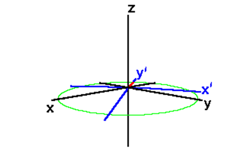
A magnetization vector rotating at the Larmor frequency in the laboratory frame appears stationary in a frame of reference rotating about the Z axis. In the rotating frame, relaxation of \(M_Z\) magnetization to its equilibrium value looks the same as it did in the laboratory frame.

A transverse magnetization vector rotating about the Z axis at the same velocity as the rotating frame will appear stationary in the rotating frame.

A magnetization vector traveling faster than the rotating frame rotates clockwise about the Z axis. A magnetization vector traveling slower than the rotating frame rotates counter-clockwise about the Z axis.


- \(\mu_{\perp}\) rotates with \(\omega_{0}\) frequency counter clockwise, while \(u\), \(v\) rotate with counter clockwise.
- \(\mu_{\parallel }\) rotates with \(\omega=\omega_{0}-\omega\) to an observer in the rotating coordinate system that rotates at the frequency \(\omega\).
Now
\[\omega_{0}=\gamma H_{\circ}-\omega_{1}=\gamma\left(H_{\circ}-\omega_{1} / \gamma\right) \nonumber \]
where the quantity in the parenthesis has the units of magnetic field. When view in the rotating coordinate system, the procession frequency is , which is what would be produce by an effective field
\[H_{e f f}=\left(H_{0}-\omega_{1} / \gamma\right) \nonumber \]
The quantity \(\omega_{1}/ \gamma\) behaves like a fictitious field that is directed in the opposite direction of \(H_o\). In vectoral units
\[\vec{H}_{e f f}=\left(H_{0}-\omega_{1} / \gamma\right) \vec{k} \nonumber \]
The equations of motion in the rotating frame are now
\[\begin{aligned}
\dot{\vec{\mu}} &=-\gamma\left[\vec{H}_{e f f} \times \vec{\mu}\right]=\\
&=-\gamma\left[\vec{H}_{\circ}-\omega_{1} / \gamma\right] \vec{k} \times \vec{\mu}
\end{aligned} \nonumber \]
As \(\omega_{1} / \gamma \rightarrow H_{0}\) or as \(\omega_{1} \rightarrow \gamma H_{0}\), the quantity in the brackets goes to zero and \(\dot{\vec{\mu}} \rightarrow 0\). Thus is stationary in a coordinate system that rotates as the Larmour frequency \(\omega_{1}=\omega_{0}\) and \(H_{e f f}=0\).
Macroscopic Statistics (magnetization)
In contrast to single molecule optical spectroscopy, the signal strength of NMR is too weak to do with a single molecule, and we need to address an ensemble of nuclei. It is cumbersome to describe NMR on a microscopic scale. A macroscopic picture is more convenient. The first step in developing the macroscopic picture is to define the spin packet. A spin packet is a group of spins experiencing the same magnetic field strength. In this example, the spins within each grid section represent a spin packet.
At any instant in time, the magnetic field due to the spins in each spin packet can be represented by a magnetization vector.

The individual for each member of the ensemble add vectorally to give a resulting bulk magnetization
\[\vec{M}=\sum_{i} \vec{\mu}_{i} \nonumber \]
The size of each vector is proportional to (N+ - N-) calculated from the Boltzman equation. The vector sum of the magnetization vectors from all of the spin packets is the net magnetization. To describe pulsed NMR, it is necessary from here on to talk in terms of the bulk or net magnetization, \(\vec{M}\).
Adapting the conventional NMR coordinate system, the external magnetic field and the net magnetization vector at equilibrium are both along the Z axis. The equation of motions for procession of \(\vec{M}\) is the same as for \(\vec{M}\).
\[\dot{\vec{M}}=-\gamma\left(H_{e f f} \times \vec{M}\right) \nonumber \]
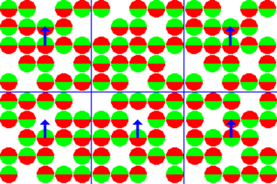
\(\vec{M}\) at equilibrium will have no x- or y- components because these average to 0 (\(\vec{\mu}_{x}\) and \(\vec{\mu}_{y}\) are random). However, an equilibrium component in the z-direction will exist, since slightly more spins will line up with \(\vec{\mu}_{z}\) (more parallel than anti parallel).
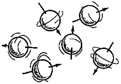
The rotation of the charged protons makes them magnetic. In the absence of field, the directions of the magnetic dipoles are random,
The equilibrium magnetization is directed along the applied magnetic field,

or as a function of all the "individual spins" looks like this:

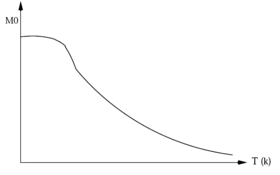
The (thermal) bulk magnetization magnitude is given by the Curie law:
\[\left|M_{0}\right|=\frac{N_{0} \mu^{2}}{3 k T} I(I+1) H_{0} \nonumber \]
At very low temperatures, only the lowest energy level is populated the magnetization given is the equilibrium magnetization inherent to a system, when placed in a magnetic Ho. It is often designated as Mo (and will be henceforth). That is, the magnetization is inversely proportional to temperature. This makes sense since the thermal motions are random and act to reduce the net magnetization of the material.