3.8: Fourier Transform IR Spectroscopy

The invention of the FFT algorithm lead to its practical application to IR Spectroscopy. Today, an inexpensive 4000-400 cm^-1 FTIR can compute a spectrum in ~0.2s. In contrast to the frequency domain spectrometers discussed in class regarding, the FTIR measures the data in time and converts it to frequency. In mathematics, Fourier analysis is a subject area which grew out of the study of Fourier series. The subject began with trying to understand when it was possible to represent general functions by sums of simpler trigonometric functions. The attempt to understand functions (or other objects) by breaking them into basic pieces that are easier to understand is one of the central themes in Fourier analysis. http://www.newport.com/store/genContent.aspx/Introduction-to-FT-IR-Spectroscopy/405840/1033

Most often, the unqualified term Fourier transform refers to the transform of functions of a continuous real argument, such as time (t). In this case the Fourier transform describes a function ƒ(t) in terms of basic complex exponentials of various frequencies. In terms of ordinary frequency ν, the Fourier transform is given by the complex number:

\[F(v)=\int_{-\infty}^{\infty} f(t) \cdot e^{-2 \pi i u t} d t \label{eq1} \]

The inverse FT is

\[f(t)=2 \pi \int_{-\infty}^{\infty} F(v) \cdot e^{+2 \pi i u t} d t \nonumber \]

There are differing expressions of this depending on how you want to normalize, or if you are talking in terms of angular frequency (\(ω\) or natural frequency \(\nu\), with \(ω=2\pi\nu\)).

The FT can be expanded into a sum of two functions: the cosine and the sine via the Euler equation:

\[e^{i x}=\cos (x)+i \sin (x) \label{Euler} \]

Combining Equations \ref{Euler} and \ref{eq1} results in

\[\begin{align*} F(v) &=\int_{-\infty}^{\infty} f(t) \cdot e^{-2 \pi i v t} d t \\[4pt] &=\int_{-\infty}^{\infty} f(t) \cdot \cos (-2 \pi v t) d t-i \int_{-\infty}^{\infty} f(t) \cdot \sin (-2 \pi v t) d t \end{align*} \nonumber \]

This can be re-written using simple trig properties (to avoid unnecessary negative signs) to

\[F(v)=\int_{-\infty}^{\infty} f(t) \cdot \cos (2 \pi v t) d t+i \int_{-\infty}^{\infty} f(t) \cdot \sin (2 \pi v t) d t \nonumber \]

What does this mean? The function \(f(t)\) can be converted from a basis that is in localized \(δ\) functions (e.g. the value of \(y\) at the exact point \(x\) with no width associated with it) to a different basis set consisting of delocalized sinusoids sines and cosines). This is a transform and there are many other basis sets out there to transform data (e.g. Lorentz transform with exponential decays or wavelets which use localized trig functions etc.).

Now back to instrumentation. How do we measure IR spectra in time? With an interferometer with works as follows.

Figure \(\PageIndex{1}\): (left) A dispersive IR instrument and (right) A FTIR instrument

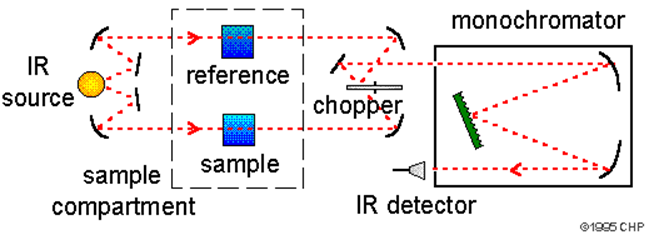
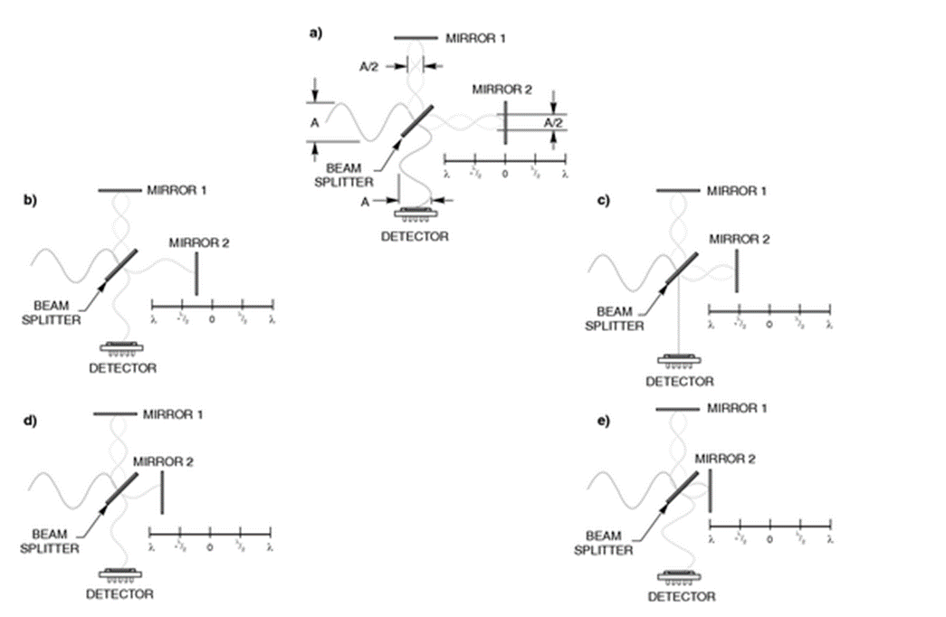
For example, a single wavelength, λ, from the source and the beam is split by a ½ reflection mirror (a beam splitter). ½ of the output goes to a stationary mirror and the other ½ goes to a moving mirror. Both halves are reflected back to the beam splitter resulting in some of the light going to the sample and detector.

Interferometer for FTIR (Public Domain; Sanchonx via Wikipedia)

If the pathlength is equal (\(δ\) = retardation = optical phase difference (OPD) = 0), then the beams (or specifically the oscillating light from each path) recombine in phase and we have a maximum at the detector (ignoring the sample). If the movable mirror is displaced by \(λ/4 =x\), then \(δ=2x= λ/2\) and the beams are out of phase and no or little light is measured at the detector. When \(δ= λ\), we have constructive interference again, etc. If we plot \(I(δ)\), the intensity measured on the detector vs. \(δ\) we get a cosine plot of wavelength \(λ\).

Figure \(\PageIndex{5}\): Schematic representation of waves and their phases, input, output, and the two arms of the interferometer as the scan goes from zero path difference condition to \(δ =λ\). (a) \(δ =0\) case. (b) \(λ/4 δ\) case. (c) \(λ/2 δ\) case. (d) \(3λ/4 δ\) case. (e) \(1λ δ\) case.

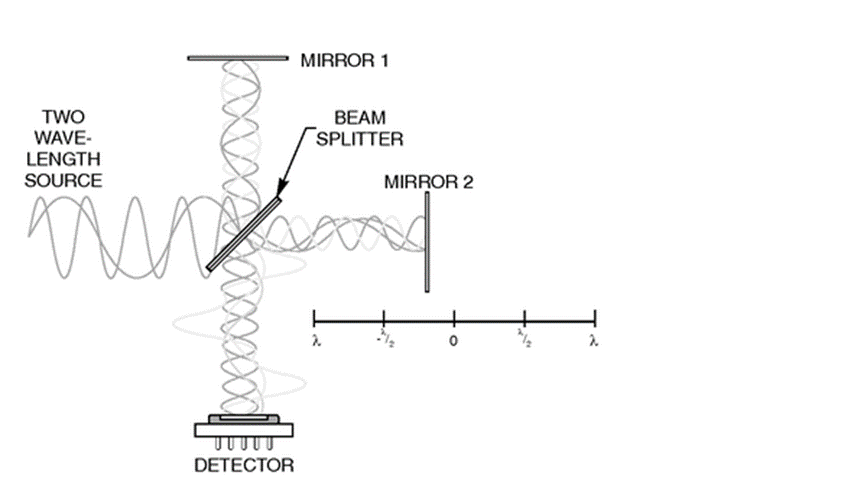
That was with one monochromatic light source, whereby physically moving the moving arm of the interferometer tells you about the wavelength of the incident light. Now what about more colors (wavelengths):

Figure \(\PageIndex{8}\): Two wavelength sources.

Now \(δ\) is the inverse of \(\tilde{\nu}\), the wavenumber of the measured light, just as velocity and time are inverses of each other. The retardation and \(\tilde{\nu}\) are relate by a Fourier Transform. Let \(B\tilde{\nu}\) be the Fourier Transform of the interferogram \(I(δ)\). (https://www.colby.edu/chemistry/NMR/...erfourier.html)

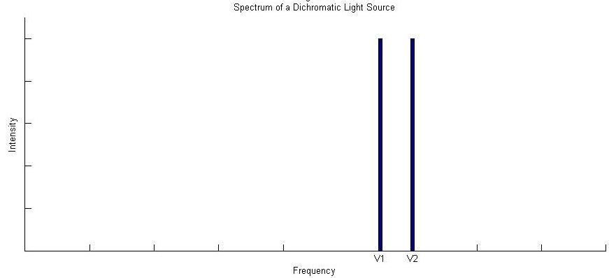
A Dichromatic FTIR Spectrometer

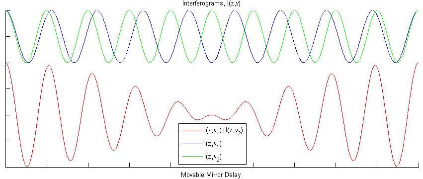
Imagine a light source that emits only two discreet frequencies of light \(\bar{ u_1}\) and \(\bar{ u_2}\) of equal intensity (Figure 1).

Figure \(\PageIndex{1}\): Dichromatic spectrum. \(\bar{ u_2} - \bar{ u_1} = 0.1\). Passing these two frequencies through the Interferometer (without an absorbing sample), and measuring the interference with a light sensitive detector gives the intensity interferogram shown in red in Figure 2. The horizontal axis in Figure two is the delay of the movable mirror in the interferometer (z), and the vertical axis is arbitrary.

Figure \(\PageIndex{2}\): Interferogram (red), and the two frequencies (blue and green). The total distance on the movable mirror delay axis is \(10\lambda_1\) or \((\lambda_2\).

Now imagine we place an absorbing sample in our interferometer, and that it absorbs light at either \(\bar{ u_1}\) or \(\bar{ u_2}\), although we do not know which one yet. The result on the measured interferogram is given in blue in Figure 3 (with the reference interferogram from Figure 2 given in green).

Figure \(\PageIndex{3}\): Interferogram with absorbing sample (blue), and background interferogram (green). Notice there is a clear difference when one of the frequencies is partially absorbed.

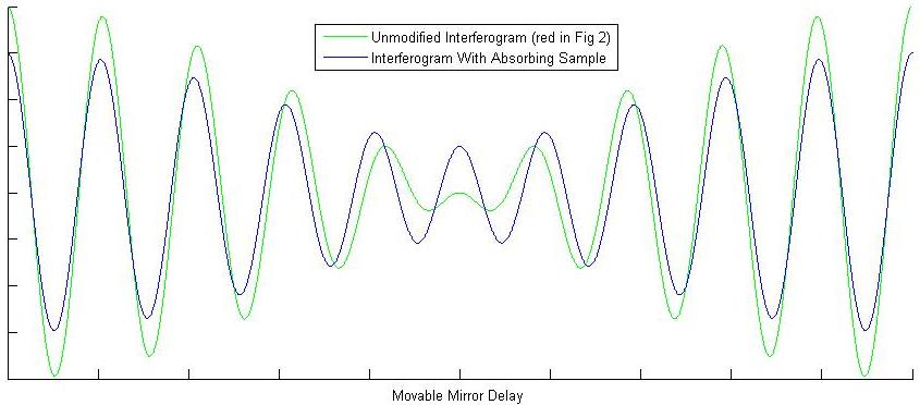
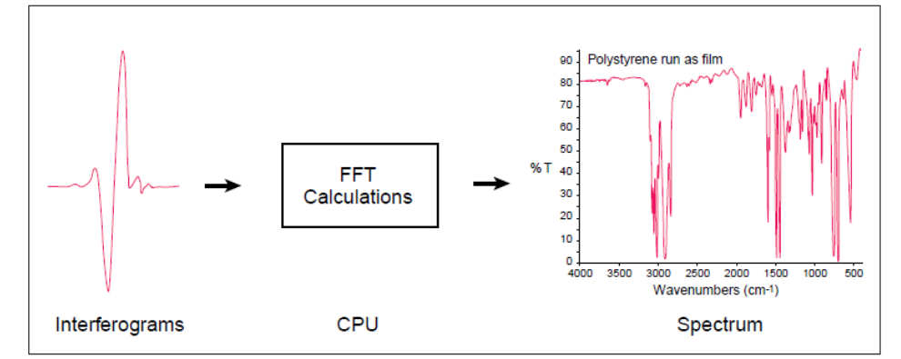
These two interferograms are all we need from the instrument! Now comes the FT of the FTIR. Fourier transforms will be covered in more detail in the next section. For now just think of it as a black box function in which you plug in an interferogram and get out a spectrum. Figure 1, therefore, is the Fourier transform of the red interferogram in Figure 2. Performing a Fourier transform on the measured blue interferogram in Figure 3 gives the spectrum in Figure 4.

Figure \(\PageIndex{4}\): Spectrum that reached the detector after the absorbing sample. This spectrum is the Fourier transform of the blue curve in Figure 3. Comparing this spectrum to the one in Figure 1 shows a clear absorption at \(\bar{ u_1}\).

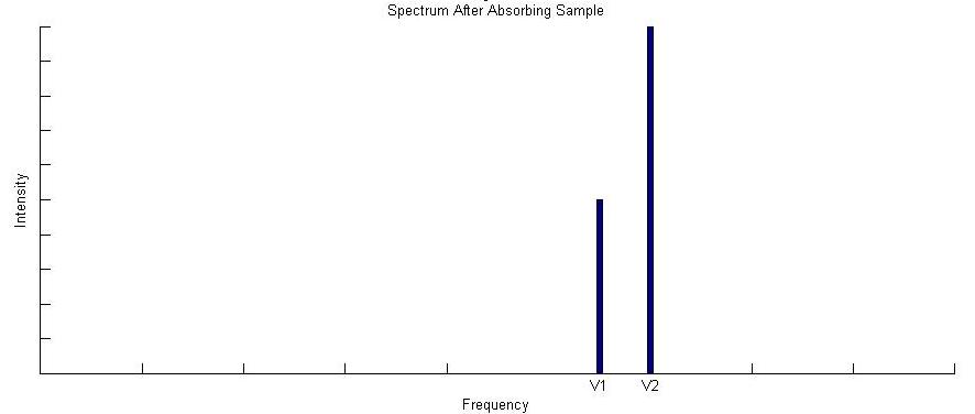
By comparing the spectrum in Figure 4 to Figure 1, we can immediately deduce that our absorbing sample absorbs light at frequency \(\bar{ u_1}\), and the FTIR spectrometer has done its job. Fundamentally thats all there is to it. The FTIR spectrometer takes light of various wavelengths, and measures an reference interferogram. You then place your absorbing sample into the interferometer and measure the interferogram again. Finally you Fourier transform both interferograms, and compare the spectra to determine what frequencies of light the sample is absorbing.

The next sections work on developing a more complete description of the the measured spectra, and the instrument nuances that factor into your data manipulation. To do this, however, we will need to open up the black box we put the Fourier transform in, and get an idea of how it works.

Fourier Transforms

From the previous section we saw that Fourier Transforms (in the context of FTIR) take an interferogram and produce a spectrum. The last section also implicitly presented the idea that the interferogram measured by an FTIR interferometer is just the sum of the interferograms of all the constituent frequencies present in the source. The Fourier transform, then, must break down the interferogram to reveal these constituent frequencies telling us which are present and in what amount.

To make this as easy on ourselves as possible, the first step we can take is to shift a maximum value of the interferogram to the origin. This ensures that it will be inherently cosine in nature (cos(0) = 1 vs sin(0)=0). As we will see in the phase error section below, this also assumes a symmetric interferogram, which you will not generally have.

Now that our interferogram is symmetric about the origin, all we need to do (all the Fourier transform does) is product it with a large variety of cosines to see which fit. The idea behind this is quite simple. If we luck out and hit our interferogram with a cosine that exactly matches one of our constituent frequencies, we will get a \(\cos^2(x)\) which is positive for all values of x. If we add up our \(\cos^2(x)\) over all values of x we will get a large positive value.

All other cosines not equal to a cosine present in the interferogram will be positive for some x and negative for the rest. Adding the positive and the negative together for all x will give zero. Lets look at the simple case of an \(\cos(x)\) interferogram tried against three different cosines and one cosine that exactly matches (Figure 5):

Figure 5a is shown. Notice that only the top (teal) curve has a large and positive area when measured over the entire window.

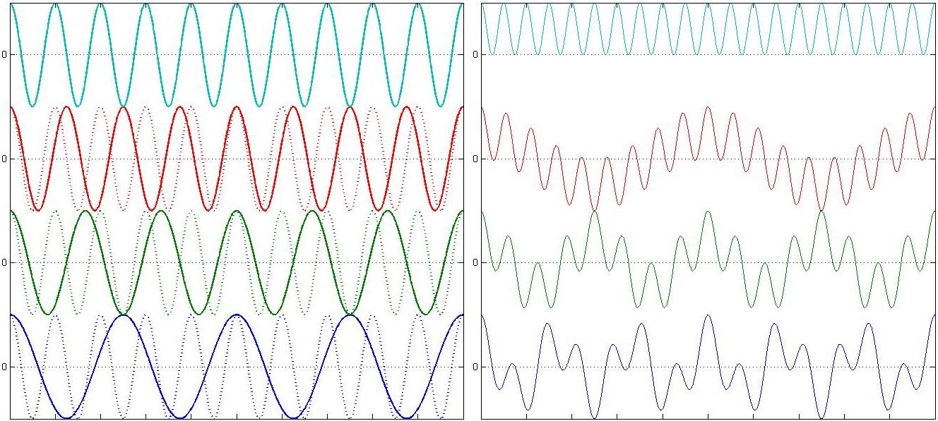
As you can see in 5b every cosine but the one that exactly matches the interferogram spends an equal amount of time above and below 0; such that if we were to add up the area under these curves, only the top (teal) one would be non-zero. We can also look at various test cosines against the interferogram from Figure 2, again ending in a cosine that matches one of the two frequencies present in that interferogram (Figure 6):

Polychromatic Light Sources

So far all we have considered are monochromatic and dichromatic FTIR spectrometers that have allowed us to use very simple interferograms. It might occur to you, however, that such instruments would not be terribly useful. We would need our samples to just happen to absorb at whatever frequency of light we selected for our interferometer. Real FTIR spectrometers don't use just two frequencies, but a whole continuum of light typically generated from a black body source (more on instrumentation here).

To get an idea of what this looks like for an interferogram lets see what happens when 5 and 50 frequencies of light interfere with equal intensities (Figure 7):

Figure 7b (right) shows the interference of 50 frequencies of with intensity.

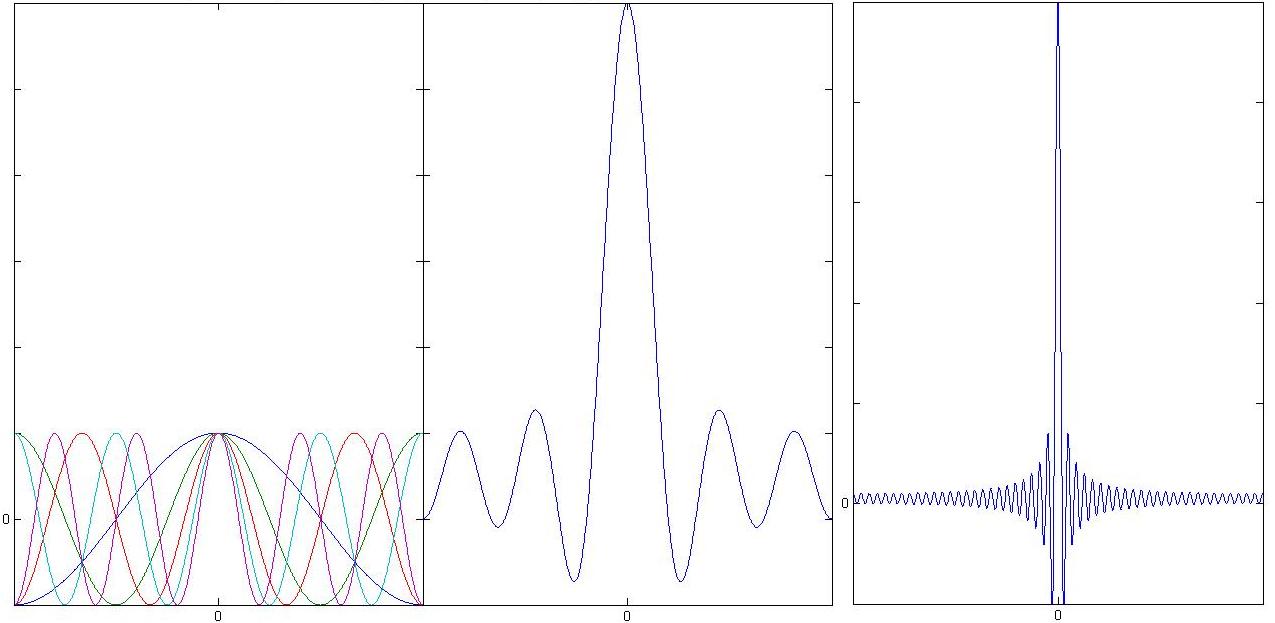
Figure 7b already has the well defined centerburst of an actual interferogram. We have, however, left out a very important feature of blackbody sources. A blackbody source emits radiation in a continuous envelope described by Planks law, and this modifies our interferogram in a significant way (Figure 8).

If the source is continuous, as in a blackbody radiator, which is usually used, then we have the cosine transform of the Fourier Transform:

\[B(\tilde{v})=\int_{-\infty}^{\infty} I(\delta) \cdot \cos (2 \pi \tilde{v} \delta) d \delta \nonumber \]

This is carried out by sampling the \(I(δ)\) through a sample window (range of δ). Then carry out the Fourier transform (or the cosine transform via the Fast Fourier Transform (FFT) algorithm.

\(\Delta \tilde{v}\) is approximated by the FFT is the emission spectrum of the source. We then put in a sample, measure an interferogram – then do a FFT and subtract the two FT’s to give the absorption spectrum by the difference.

What is the maximum frequency measured in this setup? This in Fourier Analysis is called the Nyquist wavenumber, \(\Delta \tilde{v}_n\) and is the highest frequency that you can measure in a FFT of a sample. This is given by

\[\tilde{v}_{n}=\frac{1}{2 \Delta \delta} \nonumber \]

where \(\Delta \delta\) is the retardation sampling frequency (i.e. how often you sample).

Exercise \(\PageIndex{1}\): Nyquist wavenumber

What is the ultimate resolution of \(\Delta \tilde{v}\)? Via Fourier analysis, this is giving via the length of the sampling window In this case,

\[\delta_{\max }=\Delta \nonumber \]

And the best we can do is

\[\Delta \tilde{v}=1 / \Delta. \nonumber \] Recall that time à frequency Fourier Transform:

\[\Delta \tilde{v} \propto 1 / \text { window lenth } \nonumber \]

This is the instrumentation limit in FTIR.

Example \(\PageIndex{1}\)

If

\[\delta_{\max }=\frac{1}{2} \mathrm{~cm} \nonumber \]

and this is divided into 4096 (2¹²) position slots, then

\[\delta=\frac{1}{8,000} \mathrm{~cm} \nonumber \]

and therefore

\[\tilde{v}_{n}=4000 \mathrm{~cm}^{-1}. \nonumber \]

The resolution is ~2 cm^-1.