2.14: Solvent Effect of Fluorescence

The concept of solvation can be understood from interactions between a fluorophore (the solute), and the surrounding solvent molecules. The dominating solute-solvent interactions arise from electrostatic dipole-dipole interactions, which lead to lowering the potential energies of all energy levels involved in absorption and fluorescence processes.

Figure 1: Changes in solute-solvent interactions lead to solvatochromic shifts in absorption and fluorescence spectra of the same fluorophore. (CC BY-SA-NC; Andrei Tokmakoff)

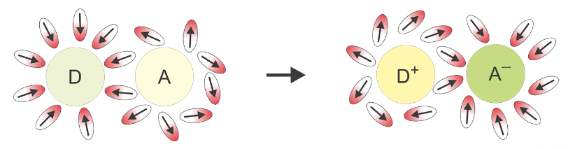
This effect can be explained by Onsager's model of solvation. According to this model, the dipole moment of the fluorophore in the ground state, \(μ_g\), interacts with the dipole moments of the surrounding solvent molecules, rearranging them in a way that minimizes the potential energy of the whole system. If we would "freeze" the molecules for a while and remove the fluorophore, the special arrangement of the solvent dipole moments would result in a non-balanced electric field \(R_g\), called the "reaction field" or "vacuum field"

Solvation Energies

In Onsager's model, the solute-solvent interaction is identified as an interaction of the fluorophore dipole moment, μ_g, with the reaction field R_g, namely:

\[U_{g}^{\text {rel }}=-\vec{\mu}_{g} \cdot \vec{R}_{g} \nonumber \]

The energy level of the ground state is therefore lowered by this value. The symbol 'rel' indicates that the solvent is in a state of thermodynamic equilibrium (relaxed).

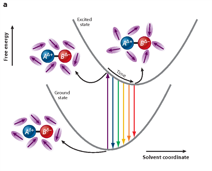
Electronic excitation of the fluorophore causes a rapid (~10^-15 s) change of its dipole moment to μ_e. This time is much too short for the solvent molecules to rearrange their orientations. Thus, immediately after excitation the interaction energy will be:

\[U_{e}^{F C}=-\vec{\mu}_{e} \cdot \vec{R}_{g} \nonumber \]

indicating that the reaction field will be still the same as it was before excitation. The symbol 'FC' indicates a non-equilibrated, Franck-Condon state. The solvent molecules need usually picoseconds (10^-12-10^-10 s) to perform solvent relaxation achieving finally the solute-solvent interaction energy (Figure 2):

\[U_{e}^{\text {rel }}=-\vec{\mu}_{e} \cdot \vec{R}_{e} \nonumber \]

Figure 2: Schematic description of the time-dependent fluorescence (TDF) process. (a) The absorption and TDF are depicted for a dye molecule, represented as A-B with a charge-transfer transition ( > δ). The purple arrows indicate solvent molecule permanent dipole moments that reorganize after excitation as measured by a collective solvent coordinate. https://www.semanticscholar.org/pape...c0d32/figure/0

The process of fluorescence brings the fluorophore dipole moment back to its ground-state value \(μ_g\), so just after fluorescence:

\[U_{e}^{F C}=-\vec{\mu}_{e} \cdot \vec{R}_{e} \nonumber \]

which finally evolves during ground-state solvent relaxation to \(U_{g}^{\text {rel }}\). Direct consequences of the different solute-solvent interaction energies at different stages of absorption and fluorescence events are the spectral shifts in absorption (\(ΔU_{abs}\) and fluorescence (\(ΔU_{flu}\)) spectra (Figure 3):

Figure 3: The typical time dependency of the fluorescence spectrum

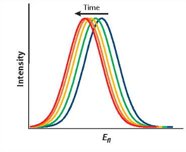
which finally evolves during ground-state solvent relaxation to \(U_{g}^{\text {rel }}\). Direct consequences of the different solute-solvent interaction energies at different stages of absorption and fluorescence events are the spectral shifts in absorption (\(ΔU_{abs}\)) and fluorescence (\(ΔU_{flu}\)) spectra:

\[\begin{aligned}
&\Delta U_{abs}=U_{e}^{F C}-U_{g}^{r e l} \\
&\Delta U_{flu}=U_{g}^{F C}-U_{e}^{r e l}
\end{aligned} \nonumber \]

Reorganization Energy

If we assume the stabilization energies in the excited and ground state are identical, we can assign them to the reorganization energy (\(\lambda\)) of the system:

\[U_{g}^{rel} = U_{e}^{r e l} = \lambda \nonumber \]

Reorganization energies are critical parameters in Marcus theory for charge transfer.