
2.10: Measures of Transition Amplitudes
- Page ID
- 364743
\( \newcommand{\vecs}[1]{\overset { \scriptstyle \rightharpoonup} {\mathbf{#1}} } \)
\( \newcommand{\vecd}[1]{\overset{-\!-\!\rightharpoonup}{\vphantom{a}\smash {#1}}} \)
\( \newcommand{\id}{\mathrm{id}}\) \( \newcommand{\Span}{\mathrm{span}}\)
( \newcommand{\kernel}{\mathrm{null}\,}\) \( \newcommand{\range}{\mathrm{range}\,}\)
\( \newcommand{\RealPart}{\mathrm{Re}}\) \( \newcommand{\ImaginaryPart}{\mathrm{Im}}\)
\( \newcommand{\Argument}{\mathrm{Arg}}\) \( \newcommand{\norm}[1]{\| #1 \|}\)
\( \newcommand{\inner}[2]{\langle #1, #2 \rangle}\)
\( \newcommand{\Span}{\mathrm{span}}\)
\( \newcommand{\id}{\mathrm{id}}\)
\( \newcommand{\Span}{\mathrm{span}}\)
\( \newcommand{\kernel}{\mathrm{null}\,}\)
\( \newcommand{\range}{\mathrm{range}\,}\)
\( \newcommand{\RealPart}{\mathrm{Re}}\)
\( \newcommand{\ImaginaryPart}{\mathrm{Im}}\)
\( \newcommand{\Argument}{\mathrm{Arg}}\)
\( \newcommand{\norm}[1]{\| #1 \|}\)
\( \newcommand{\inner}[2]{\langle #1, #2 \rangle}\)
\( \newcommand{\Span}{\mathrm{span}}\) \( \newcommand{\AA}{\unicode[.8,0]{x212B}}\)
\( \newcommand{\vectorA}[1]{\vec{#1}} % arrow\)
\( \newcommand{\vectorAt}[1]{\vec{\text{#1}}} % arrow\)
\( \newcommand{\vectorB}[1]{\overset { \scriptstyle \rightharpoonup} {\mathbf{#1}} } \)
\( \newcommand{\vectorC}[1]{\textbf{#1}} \)
\( \newcommand{\vectorD}[1]{\overrightarrow{#1}} \)
\( \newcommand{\vectorDt}[1]{\overrightarrow{\text{#1}}} \)
\( \newcommand{\vectE}[1]{\overset{-\!-\!\rightharpoonup}{\vphantom{a}\smash{\mathbf {#1}}}} \)
\( \newcommand{\vecs}[1]{\overset { \scriptstyle \rightharpoonup} {\mathbf{#1}} } \)
\( \newcommand{\vecd}[1]{\overset{-\!-\!\rightharpoonup}{\vphantom{a}\smash {#1}}} \)
\(\newcommand{\avec}{\mathbf a}\) \(\newcommand{\bvec}{\mathbf b}\) \(\newcommand{\cvec}{\mathbf c}\) \(\newcommand{\dvec}{\mathbf d}\) \(\newcommand{\dtil}{\widetilde{\mathbf d}}\) \(\newcommand{\evec}{\mathbf e}\) \(\newcommand{\fvec}{\mathbf f}\) \(\newcommand{\nvec}{\mathbf n}\) \(\newcommand{\pvec}{\mathbf p}\) \(\newcommand{\qvec}{\mathbf q}\) \(\newcommand{\svec}{\mathbf s}\) \(\newcommand{\tvec}{\mathbf t}\) \(\newcommand{\uvec}{\mathbf u}\) \(\newcommand{\vvec}{\mathbf v}\) \(\newcommand{\wvec}{\mathbf w}\) \(\newcommand{\xvec}{\mathbf x}\) \(\newcommand{\yvec}{\mathbf y}\) \(\newcommand{\zvec}{\mathbf z}\) \(\newcommand{\rvec}{\mathbf r}\) \(\newcommand{\mvec}{\mathbf m}\) \(\newcommand{\zerovec}{\mathbf 0}\) \(\newcommand{\onevec}{\mathbf 1}\) \(\newcommand{\real}{\mathbb R}\) \(\newcommand{\twovec}[2]{\left[\begin{array}{r}#1 \\ #2 \end{array}\right]}\) \(\newcommand{\ctwovec}[2]{\left[\begin{array}{c}#1 \\ #2 \end{array}\right]}\) \(\newcommand{\threevec}[3]{\left[\begin{array}{r}#1 \\ #2 \\ #3 \end{array}\right]}\) \(\newcommand{\cthreevec}[3]{\left[\begin{array}{c}#1 \\ #2 \\ #3 \end{array}\right]}\) \(\newcommand{\fourvec}[4]{\left[\begin{array}{r}#1 \\ #2 \\ #3 \\ #4 \end{array}\right]}\) \(\newcommand{\cfourvec}[4]{\left[\begin{array}{c}#1 \\ #2 \\ #3 \\ #4 \end{array}\right]}\) \(\newcommand{\fivevec}[5]{\left[\begin{array}{r}#1 \\ #2 \\ #3 \\ #4 \\ #5 \\ \end{array}\right]}\) \(\newcommand{\cfivevec}[5]{\left[\begin{array}{c}#1 \\ #2 \\ #3 \\ #4 \\ #5 \\ \end{array}\right]}\) \(\newcommand{\mattwo}[4]{\left[\begin{array}{rr}#1 \amp #2 \\ #3 \amp #4 \\ \end{array}\right]}\) \(\newcommand{\laspan}[1]{\text{Span}\{#1\}}\) \(\newcommand{\bcal}{\cal B}\) \(\newcommand{\ccal}{\cal C}\) \(\newcommand{\scal}{\cal S}\) \(\newcommand{\wcal}{\cal W}\) \(\newcommand{\ecal}{\cal E}\) \(\newcommand{\coords}[2]{\left\{#1\right\}_{#2}}\) \(\newcommand{\gray}[1]{\color{gray}{#1}}\) \(\newcommand{\lgray}[1]{\color{lightgray}{#1}}\) \(\newcommand{\rank}{\operatorname{rank}}\) \(\newcommand{\row}{\text{Row}}\) \(\newcommand{\col}{\text{Col}}\) \(\renewcommand{\row}{\text{Row}}\) \(\newcommand{\nul}{\text{Nul}}\) \(\newcommand{\var}{\text{Var}}\) \(\newcommand{\corr}{\text{corr}}\) \(\newcommand{\len}[1]{\left|#1\right|}\) \(\newcommand{\bbar}{\overline{\bvec}}\) \(\newcommand{\bhat}{\widehat{\bvec}}\) \(\newcommand{\bperp}{\bvec^\perp}\) \(\newcommand{\xhat}{\widehat{\xvec}}\) \(\newcommand{\vhat}{\widehat{\vvec}}\) \(\newcommand{\uhat}{\widehat{\uvec}}\) \(\newcommand{\what}{\widehat{\wvec}}\) \(\newcommand{\Sighat}{\widehat{\Sigma}}\) \(\newcommand{\lt}{<}\) \(\newcommand{\gt}{>}\) \(\newcommand{\amp}{&}\) \(\definecolor{fillinmathshade}{gray}{0.9}\)Now that we have looked at some of the possible electronic transitions from a theoretical point of view, we have some ammunition to assign spectra. Before we do this, we have to look at the expected intensities (strengths) of various possible absorption bands.
A convenient measure of intensity is the oscillator strength, \(f\), that is related to the integrated intensity of an absorption band.
\[f=4.314 \times 10^{-9} \int_{\text {whole band }} \varepsilon(\tilde{v}) d \tilde{v} \nonumber \]
where \(\tilde{v}\) is in units of cm-1.
For allowed electronic transitions (\(f \gt 0.1\)) and for a symmetric band shape, an approximation relation can be made that is
\[f \propto 4.6 \times 10^{-9} \varepsilon_{\max } \Delta \tilde{v}_{1 / 2} \nonumber \]
where \(\Delta \tilde{v}_{1 / 2}\) is the bandwidth at half maximum absorbance (FWHM). Typically, \(\Delta \tilde{v}_{1 / 2}=10^{3} \underline{\underline{\mathrm{cm}}^{-1}}\), so for \(f=0.1\), we have
\[0.1 \propto 4.6 \times 10^{-9} \varepsilon_{\max } 10^{3} \nonumber \]
or
\[\varepsilon_{\max }=\frac{1}{4.6 \times 10^{-5}}=2 \times 10^{4} \nonumber \]
So typically allowed electronic transitions in the UV or Vis will have \(\varepsilon_{\max } \geq 20,000\).
Transition Moment Integrals
\(f\) is related to the dipole strength, \(D\), which is the absolute squared of the transition moment integral.
\[f \propto D \equiv\left|\int_{-\infty}^{\infty} \psi_{e l} \hat{M} \psi_{e l}^{e x} d \Gamma\right|^{2}=|\langle i|\hat{M}| f\rangle|^{2} \nonumber \]
The \( \hat{M}\) operator is the important part of the \(H^{(1)}\) that appears in the Fermi golden rule. Thus, we see that f is also a measure of \(W_{i->f}\).
Above,
- \(\psi_{el}^{ex}\) or \(|f \rangle\) is the electronic wavefunction of the excited state (final),
- \(\psi_{el}\) or \(\langle i |\) is the initial electronic state.
- \( \hat{M}\) is the electric dipole moment operator and as a vectorial properties it has the components, \( \hat{M}_x\), \( \hat{M}_y\), and \( \hat{M}_z\). \( \hat{M}\) is a function of the electronic coordinates and is given by
\[\hat{M}=e \sum_{i} \vec{r}_{i} \nonumber \]
and thus each component can be calculated independently:
\[\hat{M}_{x}=e \sum_{i} x_{i} \nonumber \]
\[\hat{M}_{y}=e \sum_{i} y_{i} \nonumber \]
and
\[\hat{M}_{z}=e \sum_{i} z_{i} \nonumber \]
So the components of transform like translations along the Cartesian axis: \(x\), \(y\), \(z\). In order for a transition to be allowed by electric dipole selection rules, at least one of the following integrals must be non-zero!
\[\left\langle i\left|\hat{M}_{x}\right| f\right\rangle \label{eq1} \]
\[\left\langle i\left|\hat{M}_{y}\right| f\right\rangle \label{eq2} \]
or
\[\left\langle i\left|\hat{M}_{z}\right| f\right\rangle \label{eq3} \]
The particular transition moment integral that is not zero is an electronic transition defines the polarization of the transition. An oscillating electric field at this transition frequency aligned along the polarization axis only will induce transitions.
\[|i\rangle \rightarrow|f\rangle \nonumber \]
Sometimes transitions are forbidden by symmetry since each of the three electronic transition moment integrals is zero. Sometimes transitions will weakly occur (low f) because of small interactions such as vibronic coupling and spin-orbit coupling.
Vibronic Coupling: In this case, distortions of the molecules induce by unsymmetrical vibrations can chance the symmetry of the molecule, making an otherwise forbidden transition (for symmetry reasons) slightly allowed.
The integrand of the transition moment integral must have a component that belongs to the totally symmetric (\(A_1\) for non-centro.sym. or \(A_{1g}\) for centrosymmetric molecules) representation of the point group of the molecule. If not, the transition is symmetry forbidden.
For centrosymmetric molecules, all bands then have either a \(g\) (gerade=EVEN) or \(u\) (gerade =ODD) designation based on the character under \(i\).
For instance, \(s\) and \(d\) orbitals are \(g\) since they do not change sign under \(i\). But, \(p\) and \(f\) orbitals are \(u\) since they change sign under \(i\).
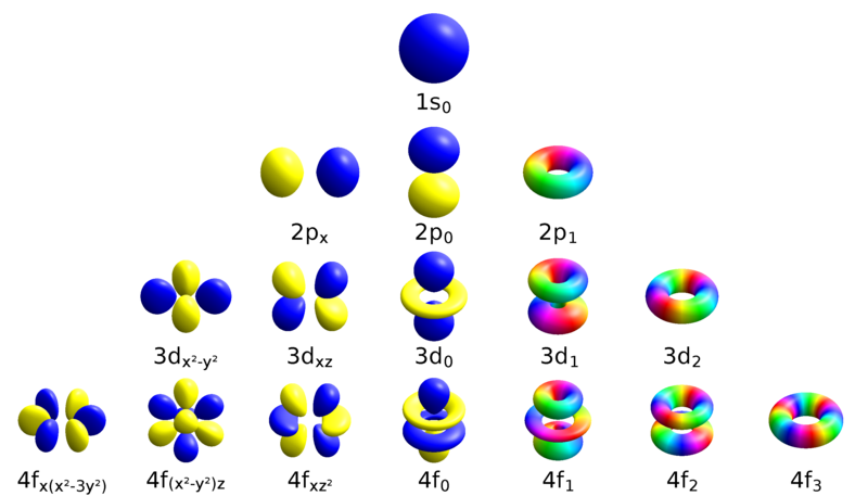
Figure: Atomic orbitals showing only the m-eigenstates. (Cc BY -SA 4.0;Geek3 via Wikipedia)
Now, \(\hat{M}_x\), \(\hat{M}_y\), and \(\hat{M}_z\) are each \(u\), so the integrands must contain \(A_{1g}\) to be allowed.
This means and thus must at least be \(g\). Now,
\[u \times u=g \times g = g \nonumber \]
and
\[u \times g=g \times u = u. \nonumber \]
Since the \(\hat{M}\) components are \(u\), then \(|i\rangle\) and \(|f\rangle\) must be \(u\) and \(g\) or \(g\) and \(u\) in order that the integrand is \(g\). Thus we get the simple LaPort rule (For centrosymmetric molecules):
\[ u \longleftrightarrow u \quad \quad \text{Transitions are forbidden} \nonumber \]
\[ g \longleftrightarrow g \quad \quad \text{Transitions are forbidden} \nonumber \]
\[ g \longleftrightarrow u \quad \quad \text{Transitions are allowed} \nonumber \]
\[ u \longleftrightarrow g \quad \quad \text{Transitions are allowed} \nonumber \]
However, the integrands must still contain the totally symeetric component (\(A_{1g}\) in this case) for it to be observed!
So for inorganic chemists in the audience, \(d \longleftrightarrow d \) electronic transitions are forbidden if the group contains \(i\) as are \(p \longleftrightarrow p \) and \(s \longleftrightarrow s \) electronic transitions etc. [Thus, for the transitions in \(\ce{Ni(H2O)6^{2+}}\) complex ion with octahedral symmetry, the \(ε\) is about 20, which is not a very intense absorption. Group has \(O_h\) symmetry and thus contains \(i\).] LaPort’s rule does say that \(p \longleftrightarrow d \) and \(s \longleftrightarrow p\) or transitions are allowed!
Transitions between states of differing spin multiplicities are forbidden. This is because the integral is evaluated over not only spatial coordinates, but also over “spin space.” does NOT contains spins variables, thus the spin integral can be separated.
So the ground-state electronic wavefunction can be written as
\[\psi_{e l}(r, s)=\psi_{e l}(r) \psi_{e l}(s) \text { or }|r, s\rangle_{e l}=|r\rangle_{e l}|s\rangle_{e l} \nonumber \]
or
and the excited state wavefunction can be similarly written as
\[\psi_{e l}^{e x}(r, s)=\psi_{e l}^{e x}(r) \psi_{e l}^{e x}(s) \text { or }|r, s\rangle_{e l}^{e x}=|r\rangle_{e l}^{e x}|s\rangle_{e l}^{e x} \nonumber \]
or
Thus the integral
\[\int_{-\infty}^{\infty} \psi_{e l}^{*} \hat{M} \psi_{e l}^{e x} d r d s=\left\langle\left. r\right|_{e l}\left\langle\left. s\right|_{e l} \hat{M} \mid r\right\rangle_{e l}^{e x} \mid s\right\rangle_{e l}^{e x}=\left\langle\left. r\right|_{e l} \hat{M} \mid r\right\rangle_{e l}^{e x}\left\langle\left. s\right|_{e l} \mid s\right\rangle_{e l}^{e x} \nonumber \]
where r represents spatial and s represents spin coordinates. If, for example, \(|r, s\rangle_{e l}\) is a singlet state and \(|r, s\rangle_{e l}^{e x}\) is a triplet state, the spin integral is
\[\left.\left\langle s \text { (singlet) }\left.\right|_{e l}\right| s(\text { triplet })\right\rangle_{e l}^{e x}=0 \nonumber \]
Since \(|r, s\rangle_{e l}\) as a single is orthogonal to \(|r, s\rangle_{e l}^{e x}\) as a triplet. However, spin-orbit coupling can mix singlet and triplet spin function together, so a weak singlet <-> triplet transition is sometimes observed. This is represented as an addition to the total Hamiltonian, \(H_{so}\), that mixes triplet wavefunctions into singlet states and vice version.