
2.1: Transition Integrals
- Page ID
- 362579
\( \newcommand{\vecs}[1]{\overset { \scriptstyle \rightharpoonup} {\mathbf{#1}} } \)
\( \newcommand{\vecd}[1]{\overset{-\!-\!\rightharpoonup}{\vphantom{a}\smash {#1}}} \)
\( \newcommand{\id}{\mathrm{id}}\) \( \newcommand{\Span}{\mathrm{span}}\)
( \newcommand{\kernel}{\mathrm{null}\,}\) \( \newcommand{\range}{\mathrm{range}\,}\)
\( \newcommand{\RealPart}{\mathrm{Re}}\) \( \newcommand{\ImaginaryPart}{\mathrm{Im}}\)
\( \newcommand{\Argument}{\mathrm{Arg}}\) \( \newcommand{\norm}[1]{\| #1 \|}\)
\( \newcommand{\inner}[2]{\langle #1, #2 \rangle}\)
\( \newcommand{\Span}{\mathrm{span}}\)
\( \newcommand{\id}{\mathrm{id}}\)
\( \newcommand{\Span}{\mathrm{span}}\)
\( \newcommand{\kernel}{\mathrm{null}\,}\)
\( \newcommand{\range}{\mathrm{range}\,}\)
\( \newcommand{\RealPart}{\mathrm{Re}}\)
\( \newcommand{\ImaginaryPart}{\mathrm{Im}}\)
\( \newcommand{\Argument}{\mathrm{Arg}}\)
\( \newcommand{\norm}[1]{\| #1 \|}\)
\( \newcommand{\inner}[2]{\langle #1, #2 \rangle}\)
\( \newcommand{\Span}{\mathrm{span}}\) \( \newcommand{\AA}{\unicode[.8,0]{x212B}}\)
\( \newcommand{\vectorA}[1]{\vec{#1}} % arrow\)
\( \newcommand{\vectorAt}[1]{\vec{\text{#1}}} % arrow\)
\( \newcommand{\vectorB}[1]{\overset { \scriptstyle \rightharpoonup} {\mathbf{#1}} } \)
\( \newcommand{\vectorC}[1]{\textbf{#1}} \)
\( \newcommand{\vectorD}[1]{\overrightarrow{#1}} \)
\( \newcommand{\vectorDt}[1]{\overrightarrow{\text{#1}}} \)
\( \newcommand{\vectE}[1]{\overset{-\!-\!\rightharpoonup}{\vphantom{a}\smash{\mathbf {#1}}}} \)
\( \newcommand{\vecs}[1]{\overset { \scriptstyle \rightharpoonup} {\mathbf{#1}} } \)
\( \newcommand{\vecd}[1]{\overset{-\!-\!\rightharpoonup}{\vphantom{a}\smash {#1}}} \)
\(\newcommand{\avec}{\mathbf a}\) \(\newcommand{\bvec}{\mathbf b}\) \(\newcommand{\cvec}{\mathbf c}\) \(\newcommand{\dvec}{\mathbf d}\) \(\newcommand{\dtil}{\widetilde{\mathbf d}}\) \(\newcommand{\evec}{\mathbf e}\) \(\newcommand{\fvec}{\mathbf f}\) \(\newcommand{\nvec}{\mathbf n}\) \(\newcommand{\pvec}{\mathbf p}\) \(\newcommand{\qvec}{\mathbf q}\) \(\newcommand{\svec}{\mathbf s}\) \(\newcommand{\tvec}{\mathbf t}\) \(\newcommand{\uvec}{\mathbf u}\) \(\newcommand{\vvec}{\mathbf v}\) \(\newcommand{\wvec}{\mathbf w}\) \(\newcommand{\xvec}{\mathbf x}\) \(\newcommand{\yvec}{\mathbf y}\) \(\newcommand{\zvec}{\mathbf z}\) \(\newcommand{\rvec}{\mathbf r}\) \(\newcommand{\mvec}{\mathbf m}\) \(\newcommand{\zerovec}{\mathbf 0}\) \(\newcommand{\onevec}{\mathbf 1}\) \(\newcommand{\real}{\mathbb R}\) \(\newcommand{\twovec}[2]{\left[\begin{array}{r}#1 \\ #2 \end{array}\right]}\) \(\newcommand{\ctwovec}[2]{\left[\begin{array}{c}#1 \\ #2 \end{array}\right]}\) \(\newcommand{\threevec}[3]{\left[\begin{array}{r}#1 \\ #2 \\ #3 \end{array}\right]}\) \(\newcommand{\cthreevec}[3]{\left[\begin{array}{c}#1 \\ #2 \\ #3 \end{array}\right]}\) \(\newcommand{\fourvec}[4]{\left[\begin{array}{r}#1 \\ #2 \\ #3 \\ #4 \end{array}\right]}\) \(\newcommand{\cfourvec}[4]{\left[\begin{array}{c}#1 \\ #2 \\ #3 \\ #4 \end{array}\right]}\) \(\newcommand{\fivevec}[5]{\left[\begin{array}{r}#1 \\ #2 \\ #3 \\ #4 \\ #5 \\ \end{array}\right]}\) \(\newcommand{\cfivevec}[5]{\left[\begin{array}{c}#1 \\ #2 \\ #3 \\ #4 \\ #5 \\ \end{array}\right]}\) \(\newcommand{\mattwo}[4]{\left[\begin{array}{rr}#1 \amp #2 \\ #3 \amp #4 \\ \end{array}\right]}\) \(\newcommand{\laspan}[1]{\text{Span}\{#1\}}\) \(\newcommand{\bcal}{\cal B}\) \(\newcommand{\ccal}{\cal C}\) \(\newcommand{\scal}{\cal S}\) \(\newcommand{\wcal}{\cal W}\) \(\newcommand{\ecal}{\cal E}\) \(\newcommand{\coords}[2]{\left\{#1\right\}_{#2}}\) \(\newcommand{\gray}[1]{\color{gray}{#1}}\) \(\newcommand{\lgray}[1]{\color{lightgray}{#1}}\) \(\newcommand{\rank}{\operatorname{rank}}\) \(\newcommand{\row}{\text{Row}}\) \(\newcommand{\col}{\text{Col}}\) \(\renewcommand{\row}{\text{Row}}\) \(\newcommand{\nul}{\text{Nul}}\) \(\newcommand{\var}{\text{Var}}\) \(\newcommand{\corr}{\text{corr}}\) \(\newcommand{\len}[1]{\left|#1\right|}\) \(\newcommand{\bbar}{\overline{\bvec}}\) \(\newcommand{\bhat}{\widehat{\bvec}}\) \(\newcommand{\bperp}{\bvec^\perp}\) \(\newcommand{\xhat}{\widehat{\xvec}}\) \(\newcommand{\vhat}{\widehat{\vvec}}\) \(\newcommand{\uhat}{\widehat{\uvec}}\) \(\newcommand{\what}{\widehat{\wvec}}\) \(\newcommand{\Sighat}{\widehat{\Sigma}}\) \(\newcommand{\lt}{<}\) \(\newcommand{\gt}{>}\) \(\newcommand{\amp}{&}\) \(\definecolor{fillinmathshade}{gray}{0.9}\)If the electronic transition dipole moment, \(\mu_{f,i}\) has a nonzero value then the particular transition can be detected by optical spectroscopy.
\[\mu_{\mathrm{f}, \mathrm{i}}=\int \Psi_{\text {final }} \hat{\mu} \Psi_{\text {initial }} \mathrm{d} \tau \neq 0 \nonumber \]
The intensities of spectroscopic transitions are proportional to the transition integral. The \(\mu\) is related to a dipole and therefore charge times distance.
\[\hat{\mu}=-e \sum_i \vec{r}_i \nonumber \]
where \(e\) is the elementary charge of an electron. Now,
\[\mu_{\mathrm{fi}}=-e \int \psi_{\text {final }} \vec{r} \psi_{\text {initial }} \mathrm{d} \tau \nonumber \]
The applicable wave functions of two states can be vibrational wave functions if we are talking about vibrational spectroscopy, electronic wave functions if we are talking about electronic spectroscopy etc.
Electronic transitions and their energetics
A diagram highlighting the various kinds of electronic excitation that may occur in organic molecules is shown below. Of the six transitions outlined, only the two lowest energy ones, \(n\) to \(\pi^{*}\) and \(\pi\) to \(\pi^{*}\) (colored blue) are achieved by the energies available in the 200 to 800 nm range of a UV/VIs spectrum. These energies are sufficient to promote or excite a molecular electron to a higher energy orbital in many conjugated compounds.
The resulting spectrum is presented as a graph of absorbance (A) versus wavelength, as in the isoprene spectrum shown below. Since isoprene is colorless, it does not absorb in the visible part of the spectrum and this region is not displayed on the graph. Notice that the convention in UV-vis spectroscopy is to show the baseline at the bottom of the graph with the peaks pointing up. Wavelength values on the x-axis are generally measured in nanometers (nm) rather than in cm-1 as is the convention in IR spectroscopy.
λmax, which is the wavelength at maximal light absorbance. As you can see, isoprene has λmax, = 222 nm. The second valuable piece of data is the absorbance at the λmax. In the isoprene spectrum the absorbance at the value λmax of 222 nm is about 0.8.
The only molecular moieties likely to absorb light in the 200 to 800 nm region are functional groups that contain pi-electrons and hetero atoms having non-bonding valence-shell electron pairs. Such light absorbing groups are referred to as chromophores. A list of some simple chromophores and their light absorption characteristics are provided below. The oxygen non-bonding electrons in alcohols and ethers do not give rise to absorption above 160 nm. Consequently, pure alcohol and ether solvents may be used for spectroscopic studies.
| Chromophore |
Example |
Excitation | λmax, nm |
ε @ λmax |
Solvent |
|---|---|---|---|---|---|
| C=C | Ethene | \(π → π^*\) | 171 | 15,000 | hexane |
| C≡C | 1-Hexyne | \(π → π^*\) | 180 | 10,000 | hexane |
| C=O | Ethanal |
\(n → π^*\) |
290 180 |
15 10,000 |
hexane hexane |
| N=O | Nitromethane |
\(n → π^*\) |
275 200 |
17 5,000 |
ethanol ethanol |
| C-X X=Br X=I |
Methyl bromide Methyl Iodide |
\(n → σ^*\) |
205 255 |
200 360 |
hexane hexane |
Electronic Transitions (cause of UV-Visible absorption)
Electronic transitions in organic molecules lead to UV and visible absorption. As a rule, energetically favored electron promotion will be from the highest occupied molecular orbital (HOMO) to the lowest unoccupied molecular orbital (LUMO), and the resulting species is called an excited state. The molecular orbital picture for the hydrogen molecule (H2) consists of one bonding σ MO, and a higher energy antibonding σ* MO. When the molecule is in the ground state, both electrons are paired in the lower-energy bonding orbital – this is the Highest Occupied Molecular Orbital (HOMO). The antibonding σ* orbital, in turn, is the Lowest Unoccupied Molecular Orbital (LUMO).
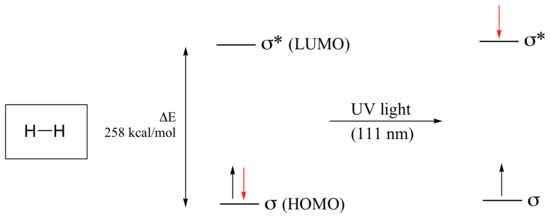
If the molecule is exposed to light of a wavelength with energy equal to ΔE, the HOMO-LUMO energy gap, this wavelength will be absorbed and the energy used to bump one of the electrons from the HOMO to the LUMO – in other words, from the σ to the σ* orbital. This is referred to as a σ - σ* transition. ΔE for this electronic transition is 258 kcal/mol, corresponding to light with a wavelength of 111 nm.
When a double-bonded molecule such as ethene (common name ethylene) absorbs light, it undergoes a π - π* transition. Because π- π* energy gaps are narrower than σ - σ* gaps, ethene absorbs light at 165 nm - a longer wavelength than molecular hydrogen.
