
16.1: All Dilute Gases Behave Ideally
- Page ID
- 57447
\( \newcommand{\vecs}[1]{\overset { \scriptstyle \rightharpoonup} {\mathbf{#1}} } \)
\( \newcommand{\vecd}[1]{\overset{-\!-\!\rightharpoonup}{\vphantom{a}\smash {#1}}} \)
\( \newcommand{\id}{\mathrm{id}}\) \( \newcommand{\Span}{\mathrm{span}}\)
( \newcommand{\kernel}{\mathrm{null}\,}\) \( \newcommand{\range}{\mathrm{range}\,}\)
\( \newcommand{\RealPart}{\mathrm{Re}}\) \( \newcommand{\ImaginaryPart}{\mathrm{Im}}\)
\( \newcommand{\Argument}{\mathrm{Arg}}\) \( \newcommand{\norm}[1]{\| #1 \|}\)
\( \newcommand{\inner}[2]{\langle #1, #2 \rangle}\)
\( \newcommand{\Span}{\mathrm{span}}\)
\( \newcommand{\id}{\mathrm{id}}\)
\( \newcommand{\Span}{\mathrm{span}}\)
\( \newcommand{\kernel}{\mathrm{null}\,}\)
\( \newcommand{\range}{\mathrm{range}\,}\)
\( \newcommand{\RealPart}{\mathrm{Re}}\)
\( \newcommand{\ImaginaryPart}{\mathrm{Im}}\)
\( \newcommand{\Argument}{\mathrm{Arg}}\)
\( \newcommand{\norm}[1]{\| #1 \|}\)
\( \newcommand{\inner}[2]{\langle #1, #2 \rangle}\)
\( \newcommand{\Span}{\mathrm{span}}\) \( \newcommand{\AA}{\unicode[.8,0]{x212B}}\)
\( \newcommand{\vectorA}[1]{\vec{#1}} % arrow\)
\( \newcommand{\vectorAt}[1]{\vec{\text{#1}}} % arrow\)
\( \newcommand{\vectorB}[1]{\overset { \scriptstyle \rightharpoonup} {\mathbf{#1}} } \)
\( \newcommand{\vectorC}[1]{\textbf{#1}} \)
\( \newcommand{\vectorD}[1]{\overrightarrow{#1}} \)
\( \newcommand{\vectorDt}[1]{\overrightarrow{\text{#1}}} \)
\( \newcommand{\vectE}[1]{\overset{-\!-\!\rightharpoonup}{\vphantom{a}\smash{\mathbf {#1}}}} \)
\( \newcommand{\vecs}[1]{\overset { \scriptstyle \rightharpoonup} {\mathbf{#1}} } \)
\( \newcommand{\vecd}[1]{\overset{-\!-\!\rightharpoonup}{\vphantom{a}\smash {#1}}} \)
\(\newcommand{\avec}{\mathbf a}\) \(\newcommand{\bvec}{\mathbf b}\) \(\newcommand{\cvec}{\mathbf c}\) \(\newcommand{\dvec}{\mathbf d}\) \(\newcommand{\dtil}{\widetilde{\mathbf d}}\) \(\newcommand{\evec}{\mathbf e}\) \(\newcommand{\fvec}{\mathbf f}\) \(\newcommand{\nvec}{\mathbf n}\) \(\newcommand{\pvec}{\mathbf p}\) \(\newcommand{\qvec}{\mathbf q}\) \(\newcommand{\svec}{\mathbf s}\) \(\newcommand{\tvec}{\mathbf t}\) \(\newcommand{\uvec}{\mathbf u}\) \(\newcommand{\vvec}{\mathbf v}\) \(\newcommand{\wvec}{\mathbf w}\) \(\newcommand{\xvec}{\mathbf x}\) \(\newcommand{\yvec}{\mathbf y}\) \(\newcommand{\zvec}{\mathbf z}\) \(\newcommand{\rvec}{\mathbf r}\) \(\newcommand{\mvec}{\mathbf m}\) \(\newcommand{\zerovec}{\mathbf 0}\) \(\newcommand{\onevec}{\mathbf 1}\) \(\newcommand{\real}{\mathbb R}\) \(\newcommand{\twovec}[2]{\left[\begin{array}{r}#1 \\ #2 \end{array}\right]}\) \(\newcommand{\ctwovec}[2]{\left[\begin{array}{c}#1 \\ #2 \end{array}\right]}\) \(\newcommand{\threevec}[3]{\left[\begin{array}{r}#1 \\ #2 \\ #3 \end{array}\right]}\) \(\newcommand{\cthreevec}[3]{\left[\begin{array}{c}#1 \\ #2 \\ #3 \end{array}\right]}\) \(\newcommand{\fourvec}[4]{\left[\begin{array}{r}#1 \\ #2 \\ #3 \\ #4 \end{array}\right]}\) \(\newcommand{\cfourvec}[4]{\left[\begin{array}{c}#1 \\ #2 \\ #3 \\ #4 \end{array}\right]}\) \(\newcommand{\fivevec}[5]{\left[\begin{array}{r}#1 \\ #2 \\ #3 \\ #4 \\ #5 \\ \end{array}\right]}\) \(\newcommand{\cfivevec}[5]{\left[\begin{array}{c}#1 \\ #2 \\ #3 \\ #4 \\ #5 \\ \end{array}\right]}\) \(\newcommand{\mattwo}[4]{\left[\begin{array}{rr}#1 \amp #2 \\ #3 \amp #4 \\ \end{array}\right]}\) \(\newcommand{\laspan}[1]{\text{Span}\{#1\}}\) \(\newcommand{\bcal}{\cal B}\) \(\newcommand{\ccal}{\cal C}\) \(\newcommand{\scal}{\cal S}\) \(\newcommand{\wcal}{\cal W}\) \(\newcommand{\ecal}{\cal E}\) \(\newcommand{\coords}[2]{\left\{#1\right\}_{#2}}\) \(\newcommand{\gray}[1]{\color{gray}{#1}}\) \(\newcommand{\lgray}[1]{\color{lightgray}{#1}}\) \(\newcommand{\rank}{\operatorname{rank}}\) \(\newcommand{\row}{\text{Row}}\) \(\newcommand{\col}{\text{Col}}\) \(\renewcommand{\row}{\text{Row}}\) \(\newcommand{\nul}{\text{Nul}}\) \(\newcommand{\var}{\text{Var}}\) \(\newcommand{\corr}{\text{corr}}\) \(\newcommand{\len}[1]{\left|#1\right|}\) \(\newcommand{\bbar}{\overline{\bvec}}\) \(\newcommand{\bhat}{\widehat{\bvec}}\) \(\newcommand{\bperp}{\bvec^\perp}\) \(\newcommand{\xhat}{\widehat{\xvec}}\) \(\newcommand{\vhat}{\widehat{\vvec}}\) \(\newcommand{\uhat}{\widehat{\uvec}}\) \(\newcommand{\what}{\widehat{\wvec}}\) \(\newcommand{\Sighat}{\widehat{\Sigma}}\) \(\newcommand{\lt}{<}\) \(\newcommand{\gt}{>}\) \(\newcommand{\amp}{&}\) \(\definecolor{fillinmathshade}{gray}{0.9}\)Ideal gases have no interactions between the particles, hence, the particles do not exert forces on each other. However, particles do experience a force when they collide with the walls of the container. Let us assume that each collision with a wall is elastic. Let us assume that the gas is in a cubic box of length \(a\) and that two of the walls are located at \(x = 0\) and at \(x = a\). Thus, a particle moving along the \(x\) direction will eventually collide with one of these walls and will exert a force on the wall when it strikes it, which we will denote as \(F_x\). Since every action has an equal and opposite reaction, the wall exerts a force \(-F_x\) on the particle.

According to Newton’s second law, the force \(-F_x\) on the particle in this direction gives rise to an acceleration via
\[-F_x = ma_x = m\dfrac{\Delta v_x}{\Delta t} \label{2.1} \]
Here, \(t\) represents the time interval between collisions with the same wall of the box. In an elastic collision, all that happens to the velocity is that it changes sign. Thus, if \(v_x\) is the velocity in the \(x\) direction before the collision, then \(-v_x\) is the velocity after, and \(\Delta v_x = -v_x - v_x = -2v_x\), so that
\[-F_x = -2m\dfrac{v_x}{\Delta t} \label{2.2} \]
Since the particles have no forces acting upon them, except for when they collide iwht the wall container, the particles move at constant speed. Thus, a collision between a particle and, say, the wall at \(x = 0\) will not change the particle’s speed. Before it strikes this wall again, it will proceed to the wall at \(x = a\) first, bounce off that wall, and then return to the wall at \(x = 0\). The total distance in the \(x\) direction traversed is \(2a\), and since the speed in the \(x\) direction is always \(v_x\), the interval \(\Delta t = \dfrac{2a}{v_x}\). Consequently, the force is:
\[-F_x = -\dfrac{mv_x^2}{a} \label{2.3} \]
Thus, the force that the particle exerts on the wall is:
\[F_x = \dfrac{mv_x^2}{a} \label{2.4} \]
The mechanical definition of pressure is the average force over area:
\[P = \dfrac{\langle F \rangle}{A} \label{2.5} \]
where \(\langle F \rangle\) is the average force exerted by all \(N\) particles on a wall of the box of area \(A\). Here \(A = a^2\). If we use the wall at \(x = 0\) we have been considering, then
\[P = \dfrac{N \langle F_x \rangle}{a^2} \label{2.6} \]
because we have \(N\) particles hitting the wall. Hence:
\[P = \dfrac{N m \langle v_x^2 \rangle}{a^3} \label{2.7} \]
from our study of the Maxwell-Boltzmann distribution, we found that:
\[\langle v_x ^2 \rangle = \dfrac{k_B T}{m} \label{2.8} \]
Hence, since \(a^3 = V\):
\[\begin{split}P &= \dfrac{N k_B T}{V} \\ &= \dfrac{n R T}{V} \label{2.9} \end{split} \]
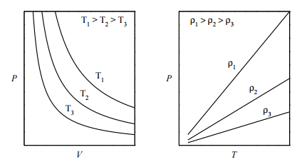
which is the ideal gas law. It relates the pressure, volume, and temperature of an ideal gas and is referred to as an equation of state. An equation of state is a relation between variables and describes the state of matter under a set of given physical conditions. One way to visualize any equation of state is to plot isotherms, which are graphs of \(P\) vs. \(V\) at fixed values of \(T\) . For the ideal-gas equation of state, some of the isotherms are shown in the figure below (left panel): If we plot \(P\) vs. \(T\) at fixed volume (called the isochores), we obtain the plot in the right panel. What is important to note, here, is that an ideal gas can exist only as a gas. It is not possible for an ideal gas to condense into some kind of “ideal liquid”. In other words, a phase transition from gas to liquid can be modeled only if interparticle interactions are properly accounted for.
We can rearrange the ideal gas equation of state to put all the constants and variables on one side:
\[\dfrac{P V}{n R T} = 1 = Z \label{2.11} \]
\(Z\) is called the compressibility of the gas. In an ideal gas, if we compress the gas by increasing \(P\) , the volume decreases as well so as to keep \(Z =1\). For a real gas, \(Z\), therefore, gives us a measure of how much the gas deviates from ideal-gas behavior.

Figure 16.1.2 shows a plot of \(Z\) vs. \(P\) for several real gases and for an ideal gas. The plot shows that for sufficiently low pressures (hence, low densities), each gas approaches ideal-gas behavior, as expected.
Extensive and Intensive Properties in Thermodynamics
Before we discuss ensembles and how we construct them, we need to introduce an important distinction between different types of thermodynamic properties that are used to characterize the ensemble. This distinction is extensive and intensive properties.
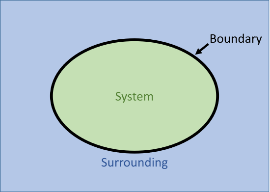
Thermodynamics always divides the universe into a system and its surroundings with a boundary between them. The unity of all three of these is the thermodynamic universe.
Now suppose we allow the system to grow in such a way that both the number of particles and the volume grow with the ratio \(N/V\) remaining constant. Any property that increases as we grow the system in this way is called an extensive property. Any property that remains the same as we grow the system in this way is called intensive.
The ideal gas equation of state can be written in an extensive form:
\[\begin{split} P V &= n R T \\ P \bar{V} &= R T \\ P &= \rho R T \label{2.10} \end{split} \]
where \(\bar{V} = V/n\) is called the molar volume and \(\rho = N/V\) is called density. Unlike \(V\) , which increases as the number of moles increases (an extensive quantity, \(\bar{V}\) and \(\rho\) do not exhibit this dependence and, therefore, are called intensive. Compressibility can also be written in an intensive form:
\[\begin{split} Z &= \dfrac{PV}{nRT} \\ &= \dfrac{P\bar{V}}{RT} \\ &= \dfrac{P}{\rho RT} \end{split} \nonumber \]
Some examples of intensive and extensive properties include:
- Extensive: number of particles (\(N\)), moles (\(n\)), volume (\(V\)), mass (\(m\)), energy, free energy
- Intensive: pressure (\(P\)), density (\(\rho\)), molar heat capacity (\(C\)), temperature (\(T\))
Contributors and Attributions
Jerry LaRue (Chapman University)