Solutions 12
- Page ID
- 47390
\( \newcommand{\vecs}[1]{\overset { \scriptstyle \rightharpoonup} {\mathbf{#1}} } \)
\( \newcommand{\vecd}[1]{\overset{-\!-\!\rightharpoonup}{\vphantom{a}\smash {#1}}} \)
\( \newcommand{\dsum}{\displaystyle\sum\limits} \)
\( \newcommand{\dint}{\displaystyle\int\limits} \)
\( \newcommand{\dlim}{\displaystyle\lim\limits} \)
\( \newcommand{\id}{\mathrm{id}}\) \( \newcommand{\Span}{\mathrm{span}}\)
( \newcommand{\kernel}{\mathrm{null}\,}\) \( \newcommand{\range}{\mathrm{range}\,}\)
\( \newcommand{\RealPart}{\mathrm{Re}}\) \( \newcommand{\ImaginaryPart}{\mathrm{Im}}\)
\( \newcommand{\Argument}{\mathrm{Arg}}\) \( \newcommand{\norm}[1]{\| #1 \|}\)
\( \newcommand{\inner}[2]{\langle #1, #2 \rangle}\)
\( \newcommand{\Span}{\mathrm{span}}\)
\( \newcommand{\id}{\mathrm{id}}\)
\( \newcommand{\Span}{\mathrm{span}}\)
\( \newcommand{\kernel}{\mathrm{null}\,}\)
\( \newcommand{\range}{\mathrm{range}\,}\)
\( \newcommand{\RealPart}{\mathrm{Re}}\)
\( \newcommand{\ImaginaryPart}{\mathrm{Im}}\)
\( \newcommand{\Argument}{\mathrm{Arg}}\)
\( \newcommand{\norm}[1]{\| #1 \|}\)
\( \newcommand{\inner}[2]{\langle #1, #2 \rangle}\)
\( \newcommand{\Span}{\mathrm{span}}\) \( \newcommand{\AA}{\unicode[.8,0]{x212B}}\)
\( \newcommand{\vectorA}[1]{\vec{#1}} % arrow\)
\( \newcommand{\vectorAt}[1]{\vec{\text{#1}}} % arrow\)
\( \newcommand{\vectorB}[1]{\overset { \scriptstyle \rightharpoonup} {\mathbf{#1}} } \)
\( \newcommand{\vectorC}[1]{\textbf{#1}} \)
\( \newcommand{\vectorD}[1]{\overrightarrow{#1}} \)
\( \newcommand{\vectorDt}[1]{\overrightarrow{\text{#1}}} \)
\( \newcommand{\vectE}[1]{\overset{-\!-\!\rightharpoonup}{\vphantom{a}\smash{\mathbf {#1}}}} \)
\( \newcommand{\vecs}[1]{\overset { \scriptstyle \rightharpoonup} {\mathbf{#1}} } \)
\(\newcommand{\longvect}{\overrightarrow}\)
\( \newcommand{\vecd}[1]{\overset{-\!-\!\rightharpoonup}{\vphantom{a}\smash {#1}}} \)
\(\newcommand{\avec}{\mathbf a}\) \(\newcommand{\bvec}{\mathbf b}\) \(\newcommand{\cvec}{\mathbf c}\) \(\newcommand{\dvec}{\mathbf d}\) \(\newcommand{\dtil}{\widetilde{\mathbf d}}\) \(\newcommand{\evec}{\mathbf e}\) \(\newcommand{\fvec}{\mathbf f}\) \(\newcommand{\nvec}{\mathbf n}\) \(\newcommand{\pvec}{\mathbf p}\) \(\newcommand{\qvec}{\mathbf q}\) \(\newcommand{\svec}{\mathbf s}\) \(\newcommand{\tvec}{\mathbf t}\) \(\newcommand{\uvec}{\mathbf u}\) \(\newcommand{\vvec}{\mathbf v}\) \(\newcommand{\wvec}{\mathbf w}\) \(\newcommand{\xvec}{\mathbf x}\) \(\newcommand{\yvec}{\mathbf y}\) \(\newcommand{\zvec}{\mathbf z}\) \(\newcommand{\rvec}{\mathbf r}\) \(\newcommand{\mvec}{\mathbf m}\) \(\newcommand{\zerovec}{\mathbf 0}\) \(\newcommand{\onevec}{\mathbf 1}\) \(\newcommand{\real}{\mathbb R}\) \(\newcommand{\twovec}[2]{\left[\begin{array}{r}#1 \\ #2 \end{array}\right]}\) \(\newcommand{\ctwovec}[2]{\left[\begin{array}{c}#1 \\ #2 \end{array}\right]}\) \(\newcommand{\threevec}[3]{\left[\begin{array}{r}#1 \\ #2 \\ #3 \end{array}\right]}\) \(\newcommand{\cthreevec}[3]{\left[\begin{array}{c}#1 \\ #2 \\ #3 \end{array}\right]}\) \(\newcommand{\fourvec}[4]{\left[\begin{array}{r}#1 \\ #2 \\ #3 \\ #4 \end{array}\right]}\) \(\newcommand{\cfourvec}[4]{\left[\begin{array}{c}#1 \\ #2 \\ #3 \\ #4 \end{array}\right]}\) \(\newcommand{\fivevec}[5]{\left[\begin{array}{r}#1 \\ #2 \\ #3 \\ #4 \\ #5 \\ \end{array}\right]}\) \(\newcommand{\cfivevec}[5]{\left[\begin{array}{c}#1 \\ #2 \\ #3 \\ #4 \\ #5 \\ \end{array}\right]}\) \(\newcommand{\mattwo}[4]{\left[\begin{array}{rr}#1 \amp #2 \\ #3 \amp #4 \\ \end{array}\right]}\) \(\newcommand{\laspan}[1]{\text{Span}\{#1\}}\) \(\newcommand{\bcal}{\cal B}\) \(\newcommand{\ccal}{\cal C}\) \(\newcommand{\scal}{\cal S}\) \(\newcommand{\wcal}{\cal W}\) \(\newcommand{\ecal}{\cal E}\) \(\newcommand{\coords}[2]{\left\{#1\right\}_{#2}}\) \(\newcommand{\gray}[1]{\color{gray}{#1}}\) \(\newcommand{\lgray}[1]{\color{lightgray}{#1}}\) \(\newcommand{\rank}{\operatorname{rank}}\) \(\newcommand{\row}{\text{Row}}\) \(\newcommand{\col}{\text{Col}}\) \(\renewcommand{\row}{\text{Row}}\) \(\newcommand{\nul}{\text{Nul}}\) \(\newcommand{\var}{\text{Var}}\) \(\newcommand{\corr}{\text{corr}}\) \(\newcommand{\len}[1]{\left|#1\right|}\) \(\newcommand{\bbar}{\overline{\bvec}}\) \(\newcommand{\bhat}{\widehat{\bvec}}\) \(\newcommand{\bperp}{\bvec^\perp}\) \(\newcommand{\xhat}{\widehat{\xvec}}\) \(\newcommand{\vhat}{\widehat{\vvec}}\) \(\newcommand{\uhat}{\widehat{\uvec}}\) \(\newcommand{\what}{\widehat{\wvec}}\) \(\newcommand{\Sighat}{\widehat{\Sigma}}\) \(\newcommand{\lt}{<}\) \(\newcommand{\gt}{>}\) \(\newcommand{\amp}{&}\) \(\definecolor{fillinmathshade}{gray}{0.9}\)Q12.1
Calculate the wavelength associated with a 42 g baseball with speed of 80 m/s.
\[\lambda = \frac{h}{p} = \frac{6.6x10^{-34}Js}{(4x10^{-2}kg)(80m/s)} = 2.06x10^{-34} m\]
Q12.2
A typical mass for a horse is 510 kg, and a typical galloping speed is 22 kilometers per hour. Use these values to answer the following questions.
- What is the momentum of a galloping horse? What is its wavelength?
- If a galloping horse's velocity and position are simultaneously measured, and the velocity is measured to within ± 1.0%, what is the uncertainty of its position?
- Suppose Planck's constant was actually 0.01 J s. How would that change your answers to (a) and (b)? Which values would be unchanged?
Hints:
- de Broglie's postulate deals with the wave-like properties of particles.
- Heisenberg's uncertainty principle deals with uncertainty of simultaneous measurements.
(a)
1. Use the relationship between velocity and momentum to find the momentum.
$$ p = m v $$
$$ p = 510\ kg \times 22\ \frac{km}{hr} \times \frac{1000\ m}{km} \times \frac{hr}{3600\ s} $$
$$ p = 3.1 \times 10^3\ \frac{kg\ m}{s} $$
2. Find the de Broglie wavelength.
$$ \lambda = \frac{h}{p} $$
$$ \lambda = \frac{6.626 \times 10^{-34}\ J\ s}{3.1 \times 10^3\ \frac{kg\ m}{s}} \times \frac{\frac{kg\ m^2}{s^2}}{J} $$
$$ \lambda = 2.1 \times 10^{-37}\ m $$
(b)
1. Find the uncertainty of momentum from the uncertainty of velocity.
$$ \Delta p = m \Delta v $$
$$ \Delta v = 0.01 \times v $$
$$ \Delta p = 510\ kg \times 0.01 \times 22\ \frac{km}{hr} \times \frac{1000\ m}{km} \times \frac{hr}{3600\ s} $$
$$ \Delta p = 31 \frac{kg\ m}{s} $$
2. Use Heisenberg's uncertainty principle to find the uncertainty of position.
$$ \Delta x \Delta p \geq \frac{h}{4 \pi} $$
$$ \Delta x \geq \frac{h}{4 \pi \Delta p} $$
$$ \Delta x \geq \frac{6.626 \times 10^{-34}\ J\ s}{4 \pi \times 3.1 \times 10^3 \frac{kg\ m}{s}} \times \frac{\frac{kg\ m^2}{s^2}}{J} $$
$$ \Delta x \geq 1.7 \times 10^{-36}\ m $$
(c)
The calculations that involve Planck's constant (h) will change. This much larger value will make the wave-like properties of the horse more important; its wavelength and uncertainty of position will increase dramatically:
$$ \lambda ' = \frac{h'}{p} = \frac{0.010\ J\ s}{3.1 \times 10^3\ \frac{kg\ m}{s} \times \frac{\frac{kg\ m^2}{s^2}}{J}} $$
$$ \lambda ' = 3.2 \times 10^{-6}\ m = 3200\ nm $$
$$ \Delta x' \geq \frac{h'}{4 \pi \Delta p} = \frac{0.010\ J\ s}{4 \pi \times 3.1 \times 10^3 \frac{kg\ m}{s}} \times \frac{\frac{kg\ m^2}{s^2}}{J} $$
$$ \Delta x' \geq 2.6 \times 10^{-5} m = 26\ \mu m $$
The momentum would not change.
Q12.3
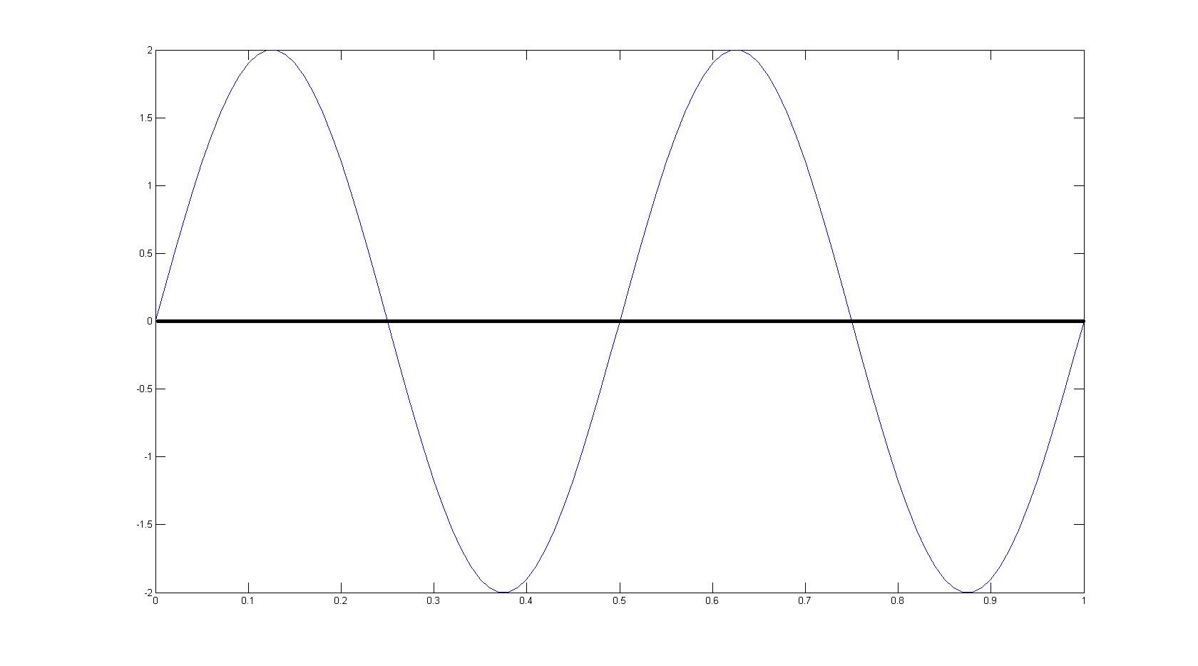
Draw the wave function for a particle in a box at the \(n = 4\) energy level.
Assuming that L = 1.

Q12.4
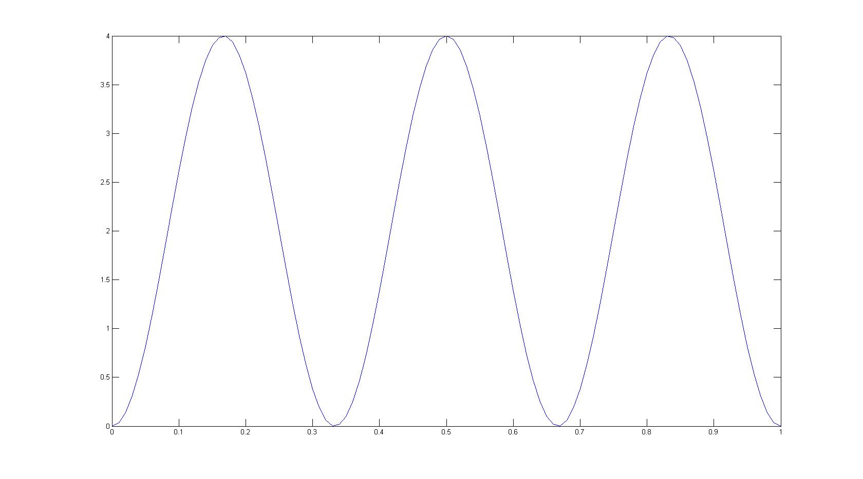
Draw the probability distribution for a particle in a box at the \(n = 3\) energy level.
Assuming that L = 1.

Q12.5
What is the probability of locating a particle of mass m between \(x = L/4\) and \(x = L/2\) in a 1-D box of length \(L\)? Assume the particle is in the \(n=1\) energy state.
To find the probability we have to integrate the n = 1 wavefunction squared from L = L/4 to L = L/2
\[P = \int_{L/4}^{L/2} \frac{2}{L}*Sin^2(\frac{\pi}{L}x)dx\]
\[P = \frac{1}{L}(\frac{L}{2} - \frac{L}{4} + \frac{L}{2\pi}) = .41\]
Q12.6
Calculate the electronic transition energy of acetylaldehyde (the stuff that gives you a hangover) using the particle in a box model. Assume that aspirin is a box of length \(300 pm\) that contains 4 electrons.
The solution to this problem depends on how many electrons can fit in each energy level of the 'box'. If we assume two, one spin up and one spin down, then the four electron occupy the n = 1 and n = 2 levels of the box with the n = 3 being the lowest unoccupied level. Therefore the first transition is from n = 2 to n = 3.
\[E_2 = \frac{4h^2}{8m(9x10^{-20})}\]
\[E_3 = \frac{9h^2}{8m(9x10^{-20})}\]
\[E_3 - E_2 = \frac{5h^2}{8m(9x10^{-20})} = 3.4x10^{-18}J = 21.2 eV\]
Q12.7
Suggest where along the box the \(n=1\) to \(n=2\) electronic transition would most likely take place.
The most likely place is where the value of the probability density of the ground state multiplied by the probabilitiy density of the excited state is a maximum.

