Solutions 3
- Page ID
- 47372
\( \newcommand{\vecs}[1]{\overset { \scriptstyle \rightharpoonup} {\mathbf{#1}} } \)
\( \newcommand{\vecd}[1]{\overset{-\!-\!\rightharpoonup}{\vphantom{a}\smash {#1}}} \)
\( \newcommand{\id}{\mathrm{id}}\) \( \newcommand{\Span}{\mathrm{span}}\)
( \newcommand{\kernel}{\mathrm{null}\,}\) \( \newcommand{\range}{\mathrm{range}\,}\)
\( \newcommand{\RealPart}{\mathrm{Re}}\) \( \newcommand{\ImaginaryPart}{\mathrm{Im}}\)
\( \newcommand{\Argument}{\mathrm{Arg}}\) \( \newcommand{\norm}[1]{\| #1 \|}\)
\( \newcommand{\inner}[2]{\langle #1, #2 \rangle}\)
\( \newcommand{\Span}{\mathrm{span}}\)
\( \newcommand{\id}{\mathrm{id}}\)
\( \newcommand{\Span}{\mathrm{span}}\)
\( \newcommand{\kernel}{\mathrm{null}\,}\)
\( \newcommand{\range}{\mathrm{range}\,}\)
\( \newcommand{\RealPart}{\mathrm{Re}}\)
\( \newcommand{\ImaginaryPart}{\mathrm{Im}}\)
\( \newcommand{\Argument}{\mathrm{Arg}}\)
\( \newcommand{\norm}[1]{\| #1 \|}\)
\( \newcommand{\inner}[2]{\langle #1, #2 \rangle}\)
\( \newcommand{\Span}{\mathrm{span}}\) \( \newcommand{\AA}{\unicode[.8,0]{x212B}}\)
\( \newcommand{\vectorA}[1]{\vec{#1}} % arrow\)
\( \newcommand{\vectorAt}[1]{\vec{\text{#1}}} % arrow\)
\( \newcommand{\vectorB}[1]{\overset { \scriptstyle \rightharpoonup} {\mathbf{#1}} } \)
\( \newcommand{\vectorC}[1]{\textbf{#1}} \)
\( \newcommand{\vectorD}[1]{\overrightarrow{#1}} \)
\( \newcommand{\vectorDt}[1]{\overrightarrow{\text{#1}}} \)
\( \newcommand{\vectE}[1]{\overset{-\!-\!\rightharpoonup}{\vphantom{a}\smash{\mathbf {#1}}}} \)
\( \newcommand{\vecs}[1]{\overset { \scriptstyle \rightharpoonup} {\mathbf{#1}} } \)
\( \newcommand{\vecd}[1]{\overset{-\!-\!\rightharpoonup}{\vphantom{a}\smash {#1}}} \)
\(\newcommand{\avec}{\mathbf a}\) \(\newcommand{\bvec}{\mathbf b}\) \(\newcommand{\cvec}{\mathbf c}\) \(\newcommand{\dvec}{\mathbf d}\) \(\newcommand{\dtil}{\widetilde{\mathbf d}}\) \(\newcommand{\evec}{\mathbf e}\) \(\newcommand{\fvec}{\mathbf f}\) \(\newcommand{\nvec}{\mathbf n}\) \(\newcommand{\pvec}{\mathbf p}\) \(\newcommand{\qvec}{\mathbf q}\) \(\newcommand{\svec}{\mathbf s}\) \(\newcommand{\tvec}{\mathbf t}\) \(\newcommand{\uvec}{\mathbf u}\) \(\newcommand{\vvec}{\mathbf v}\) \(\newcommand{\wvec}{\mathbf w}\) \(\newcommand{\xvec}{\mathbf x}\) \(\newcommand{\yvec}{\mathbf y}\) \(\newcommand{\zvec}{\mathbf z}\) \(\newcommand{\rvec}{\mathbf r}\) \(\newcommand{\mvec}{\mathbf m}\) \(\newcommand{\zerovec}{\mathbf 0}\) \(\newcommand{\onevec}{\mathbf 1}\) \(\newcommand{\real}{\mathbb R}\) \(\newcommand{\twovec}[2]{\left[\begin{array}{r}#1 \\ #2 \end{array}\right]}\) \(\newcommand{\ctwovec}[2]{\left[\begin{array}{c}#1 \\ #2 \end{array}\right]}\) \(\newcommand{\threevec}[3]{\left[\begin{array}{r}#1 \\ #2 \\ #3 \end{array}\right]}\) \(\newcommand{\cthreevec}[3]{\left[\begin{array}{c}#1 \\ #2 \\ #3 \end{array}\right]}\) \(\newcommand{\fourvec}[4]{\left[\begin{array}{r}#1 \\ #2 \\ #3 \\ #4 \end{array}\right]}\) \(\newcommand{\cfourvec}[4]{\left[\begin{array}{c}#1 \\ #2 \\ #3 \\ #4 \end{array}\right]}\) \(\newcommand{\fivevec}[5]{\left[\begin{array}{r}#1 \\ #2 \\ #3 \\ #4 \\ #5 \\ \end{array}\right]}\) \(\newcommand{\cfivevec}[5]{\left[\begin{array}{c}#1 \\ #2 \\ #3 \\ #4 \\ #5 \\ \end{array}\right]}\) \(\newcommand{\mattwo}[4]{\left[\begin{array}{rr}#1 \amp #2 \\ #3 \amp #4 \\ \end{array}\right]}\) \(\newcommand{\laspan}[1]{\text{Span}\{#1\}}\) \(\newcommand{\bcal}{\cal B}\) \(\newcommand{\ccal}{\cal C}\) \(\newcommand{\scal}{\cal S}\) \(\newcommand{\wcal}{\cal W}\) \(\newcommand{\ecal}{\cal E}\) \(\newcommand{\coords}[2]{\left\{#1\right\}_{#2}}\) \(\newcommand{\gray}[1]{\color{gray}{#1}}\) \(\newcommand{\lgray}[1]{\color{lightgray}{#1}}\) \(\newcommand{\rank}{\operatorname{rank}}\) \(\newcommand{\row}{\text{Row}}\) \(\newcommand{\col}{\text{Col}}\) \(\renewcommand{\row}{\text{Row}}\) \(\newcommand{\nul}{\text{Nul}}\) \(\newcommand{\var}{\text{Var}}\) \(\newcommand{\corr}{\text{corr}}\) \(\newcommand{\len}[1]{\left|#1\right|}\) \(\newcommand{\bbar}{\overline{\bvec}}\) \(\newcommand{\bhat}{\widehat{\bvec}}\) \(\newcommand{\bperp}{\bvec^\perp}\) \(\newcommand{\xhat}{\widehat{\xvec}}\) \(\newcommand{\vhat}{\widehat{\vvec}}\) \(\newcommand{\uhat}{\widehat{\uvec}}\) \(\newcommand{\what}{\widehat{\wvec}}\) \(\newcommand{\Sighat}{\widehat{\Sigma}}\) \(\newcommand{\lt}{<}\) \(\newcommand{\gt}{>}\) \(\newcommand{\amp}{&}\) \(\definecolor{fillinmathshade}{gray}{0.9}\)Name: ______________________________
Section: _____________________________
Student ID#:__________________________
Template:HideTOCQ3.1
Describe how graphical methods can be used to determine the order of a reaction and its rate constant from a series of data that includes the concentration of A at varying times.
If the graph of [A] versus time is linear then the reaction is zeroth order. If the plot of log of [A] versus time is linear then the reaction is first order. If the graph of one over [A] versus time is linear then the reaction is second order. The rate constant be determined from the negative value of the slope of the line of the linear graph (except for 2nd order where the rate constant is the positive value of the slope).
Q3.2 (New)
A study of the rate of the reaction represented as \(2A⟶B\) gave the following data:
| Time (s) | 0.0 | 5.0 | 10.0 | 15.0 | 20.0 | 25.0 | 35.0 |
| [A] (M) | 1.00 | 0.952 | 0.625 | 0.465 | 0.370 | 0.308 | 0.230 |
- Determine the average rate of disappearance of A between 0.0 s and 10.0 s, and between 10.0 s and 20.0 s.
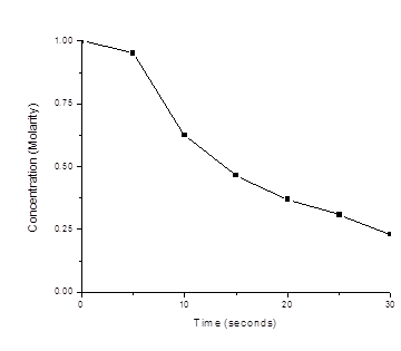
- Estimate the instantaneous rate of disappearance of A at 15.0 s from a graph of time versus [A]. What are the units of this rate?
- Use the rates found in parts (a) and (b) to determine the average rate of formation of B between 0.00 s and 10.0 s, and the instantaneous rate of formation of B at 15.0 s.
a) The average rate of disappearance from zero to ten seconds is:
\[r = -\dfrac{1.00M - 0.625\;M}{10\;s} = -0.0375 \dfrac{M}{s}\]
The average rate of disappearance from ten to twenty seconds is:
\[r = -\dfrac{0.625M - 0.370\;M}{10\;s} = -0.0255 \dfrac{M}{s}\]
b)

\[r = -.05\dfrac{M}{s}\]
c) Since it takes to 2A reactants to form a B product the rate of formation of B is negative half the rate of disappearance of A.
Q3.3
Compounds A and B both decay by first-order kinetics. The half-life of A is 20 minutes and the half-life of B is 48 minutes. If a container initially contains equal concentrations of compounds A and B, after how long will the concentration of B be twice that of A?
1. Write, in mathematical terms, the information given in the problem and what the problem is asking for.
\[ t_{1/2, A} = 20.0 min \]
\[ t_{1/2, B} = 48.0 min \]
\[ [A]_0 = [B]_0 \]
A and B decay by first-order, so
\[ -\dfrac{d[A]}{dt} = k_A [A] \]
\[ -\dfrac{d[B]}{dt} = k_B [B] \]
(Note: the rate constants for A and B are not equal, so indicate which is which with subscripts.)
Want find t at which the following is true:
\[ [B] = 2[A] \]
2. Substitute the integrated rate equations for [A] and [B]
\[ [B]_0 e^{-k_B t} = 2 [A]_0 e^{-k_A t} \]
3. Write expressions for the rate constants in terms of half-lives, and substitute into the equation.
\[ t_{1/2, A} = \dfrac{\ln2}{k_A} \Rightarrow k_A = \dfrac{\ln2}{t_{1/2, A}} \]
\[ t_{1/2, B} = \dfrac{\ln2}{k_B} \Rightarrow k_B = \dfrac{\ln2}{t_{1/2, B}} \]
\[ [B]_0 e^{-\dfrac{\ln2}{t_{1/2, B}} t} = 2 [A]_0 e^{-\dfrac{\ln2}{t_{1/2, B}} t} \]
4. Solve for t
Since initial concentrations of A and B are equal:
\[ e^{-\dfrac{\ln2}{t_{1/2, B}} t} = 2 e^{-\dfrac{\ln2}{t_{1/2, B}} t} \]
Take natural log of both sides:
\[ -\dfrac{t}{t_{1/2, B}} \ln2 = \left ( 1 - \dfrac{t}{t_{1/2, A}} \right ) \ln2 \]
\[ t = \dfrac{1}{\dfrac{1}{t_{1/2, A}} - \dfrac{1}{t_{1/2, B}}} \]
5. Plug in values for half-lives
\[t = 34.2 min\]
Answer: 34.2 minutes
Q3.4
Nitrosyl chloride, NOCl, decomposes to NO and Cl2.
\[\ce{2NOCl}(g)⟶\ce{2NO}(g)+\ce{Cl2}(g)\]
Determine the rate equation, the rate constant, and the overall order for this reaction from the following data:
| [NOCl]o (M) | 0.10 | 0.20 | 0.30 |
| Rate (mol/L/h) | 8.0 × 10⁻¹⁰ | 3.2 × 10⁻⁹ | 7.2 × 10⁻⁹ |
The general rate law for this reaction is
\[r = k[NOCl]^n \tag{3.4.1} \label{E0} \]
This equations has two unknowns at any one rate measured, so two experiments need to be measured. Let compare the initial rate for the 0.10 M and 0.20 M. From simple inspection, doubling [NOCl]o will quadruple the initial rate; this means n=2. This can be done more mathematically by taking the logarithm of the rate law (Equation \(\ref{E0}\)):
\[\ln r = n (\ln k + \ln [NOCl])\]
Now grab an experiment (e.g., middle one) and insert
\[\ln (3.2 \times 10^{-9}) = n \ln k + n \ln (0.2)\]
\[-19.56 = n \ln k - 1.61 n\]
\[\ln k = \dfrac{-19.56}{n} - 1.61 \tag{ 3.4.2} \label{E1} \]
Now we have a relationship between \(k\) and \(n\), but not either. Let's add another experiment (first one):
\[\ln (8 \times 10^{-10}) = n(\ln k + \ln (0.1))\]
\[-20.95 = n \ln k -2.30n \tag{ 3.4.3} \label{E2} \]
Now have two equations and two unknowns (it is determined). Insert Equation \(\ref{E1}\) into \(\ref{E2}\) to solve (or any other way to combine the equations):
\[-20.95 = n \left(\dfrac{-19.56}{n} - 1.61 \right) - 2.30n\]
\[-20.95 = -19.56 + 1.61n -2.30n\]
\[1.39 = 0.69n\]
Therefore.
\[n = 2\]
The reaction is second order.
Does this mean this reaction is bimolecular?
No. It means the reaction mechanism, which may involve a single bimolecular step or may not, predicts second-order kinetics.
This is an applicable was of doing this under all circumstances. For example, the intuitive double approached discussed above is hard if only considering the middle and last experiments (since the initial concentration was increased by 50%), but the math above does not care about how much it changed, as long as it was changed.
Now we know that the rate law (Equation \(\ref{E0}\)) is
\[r = k[NOCl]^2 \tag{ 3.4.4} \label{E4} \]
and \(k\) is then
\[ k = \dfrac{r}{ [NOCl]^2 }\]
Now grab an experiment and insert to \(\ref{E4}\). It doesn't matter which one (let's pick the middle one).
\[ k = \dfrac{ 3.2 \times 10^{-9} }{ 0.20^2 } = 8.0 \times 10^{−8} \;L/mol/s \]
or the first one
\[ k = \dfrac{ 8 \times 10^{-10} }{ 0.10^2 } = 8.0 \times 10^{−8} \;L/mol/s \]
or the last one
\[ k = \dfrac{ 7.2 \times 10^{-9} }{ 0.30^2 } = 8.0 \times 10^{−8} \;L/mol/s \]
Warning: In the lab, these will rarely give identical results and a fit to the data is required (since the data overdetermines the unknowns, as it always should).
Q3.5
Hydrogen reacts with nitrogen monoxide to form dinitrogen monoxide (laughing gas) according to the equation:
\[\ce{H2}(g)+\ce{2NO}(g)⟶\ce{N2O}(g)+\ce{H2O}(g)\]
Determine the rate equation, the rate constant, and the orders with respect to each reactant from the following data:
| [NO] (M) | 0.30 | 0.60 | 0.60 |
| [H2] (M) | 0.35 | 0.35 | 0.70 |
| Rate (mol/L/s) | 2.835 × 10⁻³ | 1.134 × 10⁻² | 2.268 × 10⁻² |
The general rate law for this reaction is
\[r = k[H_2]^n[NO]^m\]
This equations has three unknowns at any one rate measured, so three experiments need to be measured (and was). Let compare the initial rate for the first two experiments. From simple inspection, doubling [NO] quadruple the initial rate; this means m=2. Comparing the last two experiments shows that doubling [H2] doubles the rate n =1. This can be done more mathematically:
\[2.835\times 10^{-3} = k[H_2]^n[0.3]^m \tag{3.5.2} \]
\[1.134\times 10^{-2} = k[H_2]^n[0.6]^m \tag{3.5.2} \]
\[\dfrac{(1)}{(2)} = 0.25 = \dfrac{[0.3]^m}{[0.6]^m}\]
\[-1.39 = m(\ln(0.3) - \ln(0.6))\]
Therefore
\[m = 2\]
\[1.134\times 10^{-2} = k[0.35]^n[NO]^m \tag{3.5.3} \]
\[2.268\times 10^{-2} = k[0.7]^n[NO]^m \tag{3.5.4} \]
\[\dfrac{(3)}{(4)} = 0.5 = \dfrac{[0.35]^n}{[0.7]^n}\]
\[-0.69 = m(\ln(0.35) - \ln(0.7))\]
Therefore
\[n = 1\]
Inserting an experiment (e.g., the middle one) into the rate law will allow the determination of the rate constants.
\[1.134 \times 10^{-2} = k[0.35][0.6]^2\]
\[k = 0.09 \; M^{-2} s^{-1}\]
Note: always make sure the units of the rate constant makes sense from a dimensional analysis.
Q3.6
Use the data provided to graphically determine the order and rate constant of the following reaction:
\[\ce{SO2Cl2 ⟶ SO2 + Cl2}\]
| Time (s) | 0 | 5.00 × 10³ | 1.00 × 10⁴ | 1.50 × 10⁴ | 2.50 × 10⁴ | 3.00 × 10⁴ | 4.00 × 10⁴ |
| [SO2Cl2] (M) | 0.100 | 0.0896 | 0.0802 | 0.0719 | 0.0577 | 0.0517 | 0.0415 |
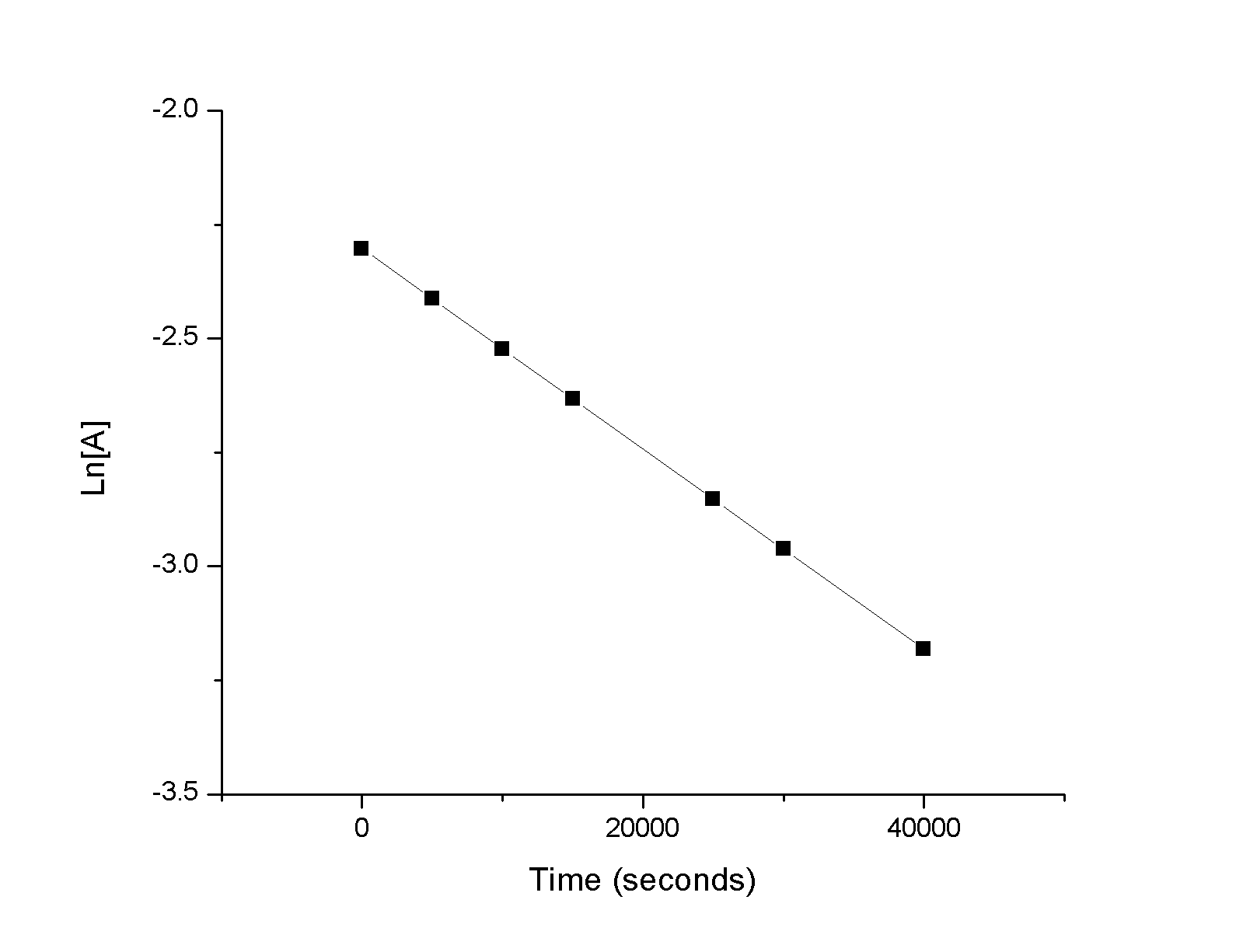
Looking at the graph above it is clear that the reaction is first order as the \(\ln[A]\) vs. time plot is linear. The slope of the line is \(-2.2\times 10^{-5}\) and thus \(k = 2.2\times 10^{-5}\).
Q3.7
Some bacteria are resistant to the antibiotic penicillin because they produce penicillinase, an enzyme with a molecular weight of 3 × 10⁴ g/mol that converts penicillin into inactive molecules. Although the kinetics of enzyme-catalyzed reactions can be complex, at low concentrations this reaction can be described by a rate equation that is first order in the catalyst (penicillinase) and that also involves the concentration of penicillin. From the following data: 1.0 L of a solution containing 0.15 µg (0.15 × 10⁻⁶ g) of penicillinase, determine the order of the reaction with respect to penicillin and the value of the rate constant.
| [Penicillin] (M) | Rate (mol/L/min) |
|---|---|
| 2.0 × 10⁻⁶ | 1.0 × 10⁻¹⁰ |
| 3.0 × 10⁻⁶ | 1.5 × 10⁻¹⁰ |
| 4.0 × 10⁻⁶ | 2.0 × 10⁻¹⁰ |
\[1\times 10^{-10} = k[5\times 10^{-12}][2\times 10^{-6}]^m \tag{3.6.1}\]
\[1\times 10^{-10} = k[5\times 10^{-12}][3\times 10^{-6}]^m \tag{3.6.2} \]
\[\dfrac{(1)}{(2)} = \dfrac{2}{3} = \dfrac{[2\times 10^{-6}]^m}{[3\times 10^{-6}]^m}\]
Taking the natural log of both sides
\[-0.405 = m(-13.12 + 12.72)\]
\[m = 1\]
\[1\times 10^{-10} = k[[5\times 10^{-12}][2\times 10^{-6}]\]
\[k = 1\times 10^7\]


