4.7: The Schrödinger Wave Equation
- Page ID
- 20295
\( \newcommand{\vecs}[1]{\overset { \scriptstyle \rightharpoonup} {\mathbf{#1}} } \)
\( \newcommand{\vecd}[1]{\overset{-\!-\!\rightharpoonup}{\vphantom{a}\smash {#1}}} \)
\( \newcommand{\id}{\mathrm{id}}\) \( \newcommand{\Span}{\mathrm{span}}\)
( \newcommand{\kernel}{\mathrm{null}\,}\) \( \newcommand{\range}{\mathrm{range}\,}\)
\( \newcommand{\RealPart}{\mathrm{Re}}\) \( \newcommand{\ImaginaryPart}{\mathrm{Im}}\)
\( \newcommand{\Argument}{\mathrm{Arg}}\) \( \newcommand{\norm}[1]{\| #1 \|}\)
\( \newcommand{\inner}[2]{\langle #1, #2 \rangle}\)
\( \newcommand{\Span}{\mathrm{span}}\)
\( \newcommand{\id}{\mathrm{id}}\)
\( \newcommand{\Span}{\mathrm{span}}\)
\( \newcommand{\kernel}{\mathrm{null}\,}\)
\( \newcommand{\range}{\mathrm{range}\,}\)
\( \newcommand{\RealPart}{\mathrm{Re}}\)
\( \newcommand{\ImaginaryPart}{\mathrm{Im}}\)
\( \newcommand{\Argument}{\mathrm{Arg}}\)
\( \newcommand{\norm}[1]{\| #1 \|}\)
\( \newcommand{\inner}[2]{\langle #1, #2 \rangle}\)
\( \newcommand{\Span}{\mathrm{span}}\) \( \newcommand{\AA}{\unicode[.8,0]{x212B}}\)
\( \newcommand{\vectorA}[1]{\vec{#1}} % arrow\)
\( \newcommand{\vectorAt}[1]{\vec{\text{#1}}} % arrow\)
\( \newcommand{\vectorB}[1]{\overset { \scriptstyle \rightharpoonup} {\mathbf{#1}} } \)
\( \newcommand{\vectorC}[1]{\textbf{#1}} \)
\( \newcommand{\vectorD}[1]{\overrightarrow{#1}} \)
\( \newcommand{\vectorDt}[1]{\overrightarrow{\text{#1}}} \)
\( \newcommand{\vectE}[1]{\overset{-\!-\!\rightharpoonup}{\vphantom{a}\smash{\mathbf {#1}}}} \)
\( \newcommand{\vecs}[1]{\overset { \scriptstyle \rightharpoonup} {\mathbf{#1}} } \)
\( \newcommand{\vecd}[1]{\overset{-\!-\!\rightharpoonup}{\vphantom{a}\smash {#1}}} \)
\(\newcommand{\avec}{\mathbf a}\) \(\newcommand{\bvec}{\mathbf b}\) \(\newcommand{\cvec}{\mathbf c}\) \(\newcommand{\dvec}{\mathbf d}\) \(\newcommand{\dtil}{\widetilde{\mathbf d}}\) \(\newcommand{\evec}{\mathbf e}\) \(\newcommand{\fvec}{\mathbf f}\) \(\newcommand{\nvec}{\mathbf n}\) \(\newcommand{\pvec}{\mathbf p}\) \(\newcommand{\qvec}{\mathbf q}\) \(\newcommand{\svec}{\mathbf s}\) \(\newcommand{\tvec}{\mathbf t}\) \(\newcommand{\uvec}{\mathbf u}\) \(\newcommand{\vvec}{\mathbf v}\) \(\newcommand{\wvec}{\mathbf w}\) \(\newcommand{\xvec}{\mathbf x}\) \(\newcommand{\yvec}{\mathbf y}\) \(\newcommand{\zvec}{\mathbf z}\) \(\newcommand{\rvec}{\mathbf r}\) \(\newcommand{\mvec}{\mathbf m}\) \(\newcommand{\zerovec}{\mathbf 0}\) \(\newcommand{\onevec}{\mathbf 1}\) \(\newcommand{\real}{\mathbb R}\) \(\newcommand{\twovec}[2]{\left[\begin{array}{r}#1 \\ #2 \end{array}\right]}\) \(\newcommand{\ctwovec}[2]{\left[\begin{array}{c}#1 \\ #2 \end{array}\right]}\) \(\newcommand{\threevec}[3]{\left[\begin{array}{r}#1 \\ #2 \\ #3 \end{array}\right]}\) \(\newcommand{\cthreevec}[3]{\left[\begin{array}{c}#1 \\ #2 \\ #3 \end{array}\right]}\) \(\newcommand{\fourvec}[4]{\left[\begin{array}{r}#1 \\ #2 \\ #3 \\ #4 \end{array}\right]}\) \(\newcommand{\cfourvec}[4]{\left[\begin{array}{c}#1 \\ #2 \\ #3 \\ #4 \end{array}\right]}\) \(\newcommand{\fivevec}[5]{\left[\begin{array}{r}#1 \\ #2 \\ #3 \\ #4 \\ #5 \\ \end{array}\right]}\) \(\newcommand{\cfivevec}[5]{\left[\begin{array}{c}#1 \\ #2 \\ #3 \\ #4 \\ #5 \\ \end{array}\right]}\) \(\newcommand{\mattwo}[4]{\left[\begin{array}{rr}#1 \amp #2 \\ #3 \amp #4 \\ \end{array}\right]}\) \(\newcommand{\laspan}[1]{\text{Span}\{#1\}}\) \(\newcommand{\bcal}{\cal B}\) \(\newcommand{\ccal}{\cal C}\) \(\newcommand{\scal}{\cal S}\) \(\newcommand{\wcal}{\cal W}\) \(\newcommand{\ecal}{\cal E}\) \(\newcommand{\coords}[2]{\left\{#1\right\}_{#2}}\) \(\newcommand{\gray}[1]{\color{gray}{#1}}\) \(\newcommand{\lgray}[1]{\color{lightgray}{#1}}\) \(\newcommand{\rank}{\operatorname{rank}}\) \(\newcommand{\row}{\text{Row}}\) \(\newcommand{\col}{\text{Col}}\) \(\renewcommand{\row}{\text{Row}}\) \(\newcommand{\nul}{\text{Nul}}\) \(\newcommand{\var}{\text{Var}}\) \(\newcommand{\corr}{\text{corr}}\) \(\newcommand{\len}[1]{\left|#1\right|}\) \(\newcommand{\bbar}{\overline{\bvec}}\) \(\newcommand{\bhat}{\widehat{\bvec}}\) \(\newcommand{\bperp}{\bvec^\perp}\) \(\newcommand{\xhat}{\widehat{\xvec}}\) \(\newcommand{\vhat}{\widehat{\vvec}}\) \(\newcommand{\uhat}{\widehat{\uvec}}\) \(\newcommand{\what}{\widehat{\wvec}}\) \(\newcommand{\Sighat}{\widehat{\Sigma}}\) \(\newcommand{\lt}{<}\) \(\newcommand{\gt}{>}\) \(\newcommand{\amp}{&}\) \(\definecolor{fillinmathshade}{gray}{0.9}\)Beginning in the early 20th century, physicists began to acknowledge that matter--much like electromagnetic radiation--possessed wave-like behaviors. While electromagnetic radiation were well understood to obey Maxwell's Equations, matter obeyed no known equations.
Introduction
In 1926, the Austrian physicist Erwin Schrödinger formulated what came to be known as the (time-dependent) Schrödinger Equation:
\[ i\hbar\dfrac{\partial}{\partial t}\Psi(x,t)=\dfrac{-\hbar}{2m}\nabla^2\Psi(x,t) +V(x)\Psi(x,t) \label{1.1}\]
Equation \(\ref{1.1}\) effectively describes matter as a wave that fluctuates with both displacement and time. Since the imaginary portion of the equation dictates its time dependence, it is sufficed to say that for most purposes it can be treated as time-independent. The result is seen in Equation \(\ref{1.3}\):
\[\dfrac{-\hbar^2}{2m}\dfrac{d^2\psi(x)}{dx^2}+V(x)\psi(x) = E\psi(x) \label{1.3}\]
Although this time-independent Schrödinger Equation can be useful to describe a matter wave in free space, we are most interested in waves when confined to a small region, such as an electron confined in a small region around the nucleus of an atom. Several different models have been developed that provide a means by which to study a matter-wave when confined to a small region: the particle in a box (infinite well), finite well, and the Hydrogen atom. We will discuss each of these in order to develop a greater understanding for how a wave behaves when it is in a bound state.


There are four general aspects that are applicable to an acceptable wavefunction
- An acceptable wavefunction will be the solution of the Schrödinger equation (either Equations \(\ref{1.1}\) or \(\ref{1.3}\)).
- An acceptable wavefunction must be normalizable so will approaches zero as position approaches infinity.
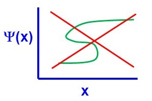
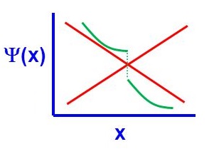
- An acceptable wavefunction must be a continuous function of position.
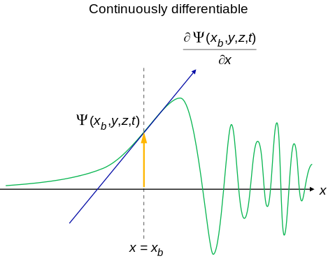
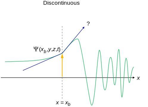
- An acceptable wavefunction will have a continuous slope (Figure \(\PageIndex{1}\)).


Interpretation of the Wavefunction
Since wavefunctions can in general be complex functions, the physical significance cannot be found from the function itself because the \(\sqrt {-1}\) is not a property of the physical world. Rather, the physical significance is found in the product of the wavefunction and its complex conjugate, i.e. the absolute square of the wavefunction, which also is called the square of the modulus.
\[ \psi ^* (r , t ) \psi (r , t ) = {|\psi (r , t ) |}^2 \label{3-34}\]
where \(r\) is a vector (x, y, z) specifying a point in three-dimensional space. The square is used, rather than the modulus itself, just like the intensity of a light wave depends on the square of the electric field. At one time it was thought that for an electron described by the wavefunction \(\psi(r)\), the quantity \(e\psi^*(r_i)\psi(r_i)d\tau\) was the amount of charge to be found in the volume \(d\tau\) located at \(r_i\). However, Max Born found this interpretation to be inconsistent with the results of experiments.
The Born interpretation, which generally is accepted today, is that \(\psi^*(r_i)\psi(r_i)\, d\tau\) is the probability that the electron is in the volume dτ located at \(r_i\). The Born interpretation therefore calls the wavefunction the probability amplitude, the absolute square of the wavefunction is called the probability density, and the probability density times a volume element in three-dimensional space (\(d\tau\)) is the probability. The idea that we can understand the world of atoms and molecules only in terms of probabilities is disturbing to some, who are seeking more satisfying descriptions through ongoing research.
Normalization of the Wavefunction
A probability is a real number between 0 and 1. An outcome of a measurement which has a probability 0 is an impossible outcome, whereas an outcome which has a probability 1 is a certain outcome. The probability of a measurement of \(x\) yielding a result between \(-\infty\) and \(+\infty\) is
\[P_{x \in -\infty:\infty}(t) = \int_{-\infty}^{\infty}\vert\psi(x,t)\vert^{ 2} dx. \label{3.6.2}\]
However, a measurement of \(x\) must yield a value between \(-\infty\) and \(+\infty\), since the particle has to be located somewhere. It follows that \(P_{x \in -\infty:\infty}(t) =1\), or
\[\int_{-\infty}^{\infty}\vert\psi(x,t)\vert^{ 2} dx = 1, \label{3.6.3}\]
which is generally known as the normalization condition for the wavefunction.
Example \(\PageIndex{1}\): Normalizing a Gaussian wavefunction
Normalize the wavefunction of a Gaussian wave packet, centered on \(x=x_o\), and of characteristic width \(\sigma\): i.e.,
\[\psi(x) = \psi_0 {\rm e}^{-(x-x_0)^{ 2}/(4 \sigma^2)}. \label{3.6.4}\]
Solution
To determine the normalization constant \(\psi_0\), we simply substitute Equation \(\ref{3.6.4}\) into Equation \(\ref{3.6.3}\), to obtain
\[\vert\psi_0\vert^{ 2}\int_{-\infty}^{\infty}{\rm e}^{-(x-x_0)^{ 2}/(2 \sigma^2)} dx = 1. \label{3.6.5}\]
Changing the variable of integration to \(y=(x-x_0)/(\sqrt{2} \sigma)\), we get
\[\vert\psi_0\vert^{ 2}\sqrt{2} \sigma \int_{-\infty}^{\infty}{\rm e}^{-y^2} dy=1. \label{3.6.6}\]
However,
\[\int_{-\infty}^{\infty}{\rm e}^{-y^2} dy = \sqrt{\pi}, \label{3.6.7}\]
which implies that
\[\vert\psi_0\vert^{ 2} = \dfrac{1}{(2\pi \sigma^2)^{1/2}}. \label{3.6.8}\]
Hence, a general normalized Gaussian wavefunction takes the form
\[\psi(x) = \dfrac{e^{\rm{i} \phi}}{(2\pi \sigma^2)^{1/4}}e^{-(x-x_0)^2/(4 \sigma^2)} \label{3.6.9}\]
where \(\phi\) is an arbitrary real phase-angle.
Contributors and Attributions
David M. Hanson, Erica Harvey, Robert Sweeney, Theresa Julia Zielinski ("Quantum States of Atoms and Molecules")

