8.7: Bond Polarity and Electronegativity

Introduction

In a covalent bond electrons are shared in a bonding orbital between two nuclei. If it is a homonuclear bond (between atoms of the same element like in H₂, N₂, O₂, Cl₂,...), the bonding electrons are shared equally and the charge distribution around the bond is symmetric. If it is a heteronuclear bond like H-Cl or H-C, the electrons may or may not be shared equally. Equally shared electrons result in a non-polar bond and unequally shared electrons result in a polar bond, where one atom feels a partially positive charge (\(\delta ^{+}\)) and the other atom feels a partially negative charge (\(\delta ^{-}\)). We will introduce the concept of electronegativity (\(\chi\), pronounced "ky" as in "sky") to help identify if a bond is polar or not, with bonding atoms with a higher electronegativity attracting electron density more than atoms with a lower electronegativty.

Orbitals of two atoms of similar electronegativity come come together to form a symmetric nonpolar covalent bond	Orbitals of two atoms of dissimilar electronegativity come together and form an asymmetric polar covalent bond.

Figure \(\PageIndex{1}\) : The atoms of the left have equal electronegativity and so form a nonpolar bond with a symmetric electron distribution. The atoms on the right have different electronegativity, with the pink orbital having a higher electronegativity than the blue, and so the resulting bond is assymetric, with there being a partial negative charge on the more electronegative atom and a partial positive on the less electronegative atom.

In Summary:

• A nonpolar covalent bond has a symmetric bonding orbital electron density function with equal sharing of the bonding electron.
• A polar covalent bond has an asymmetric bonding orbital electron density function with non-equal sharing of the bonding electrons

Electronegativity

Introduction

Electronegativity is not a thermodynamic property and has no units. The term "electronegativity" was introduced by Berzelius in 1811 and we will use the Pauling scale for electronegativities, developed by Linus Pauling, which ranges in value from 0.7 (Francium and Cesium) to 4.0 (Fluorine). Although we assign electronegativity values to element, they are not properties of an atoms per se, but of the atoms when in a bond. That is, if two atoms of different electronegativities form a bond, the more electronegative element will pull electron density from the less electronegative element, which can also be classified as the more electropositive element. It also needs to be noted that in a molecule where an atom is bonded to more than one other atom, the actual electron distribution is the result of all interactions.

Periodic Trends of Electronegativities

On a basic level, electronegativities can be correlated to ionization energies and electron affinities, although the later are thermodynamic properties of an isolated atom in the gas phase, while electronegativities are based on an arbitrary unitless scale, and there is no way you could calculate them from thermodynamic data. That said, atoms with low ionization energies (which are always endothermic) tend to be electropositive, because they do not tightly hold onto their valence electrons. Likewise, atoms with exothermic electron affinities (release energy when they gain an electron) tend to have high electron energies as they like to gain electrons.

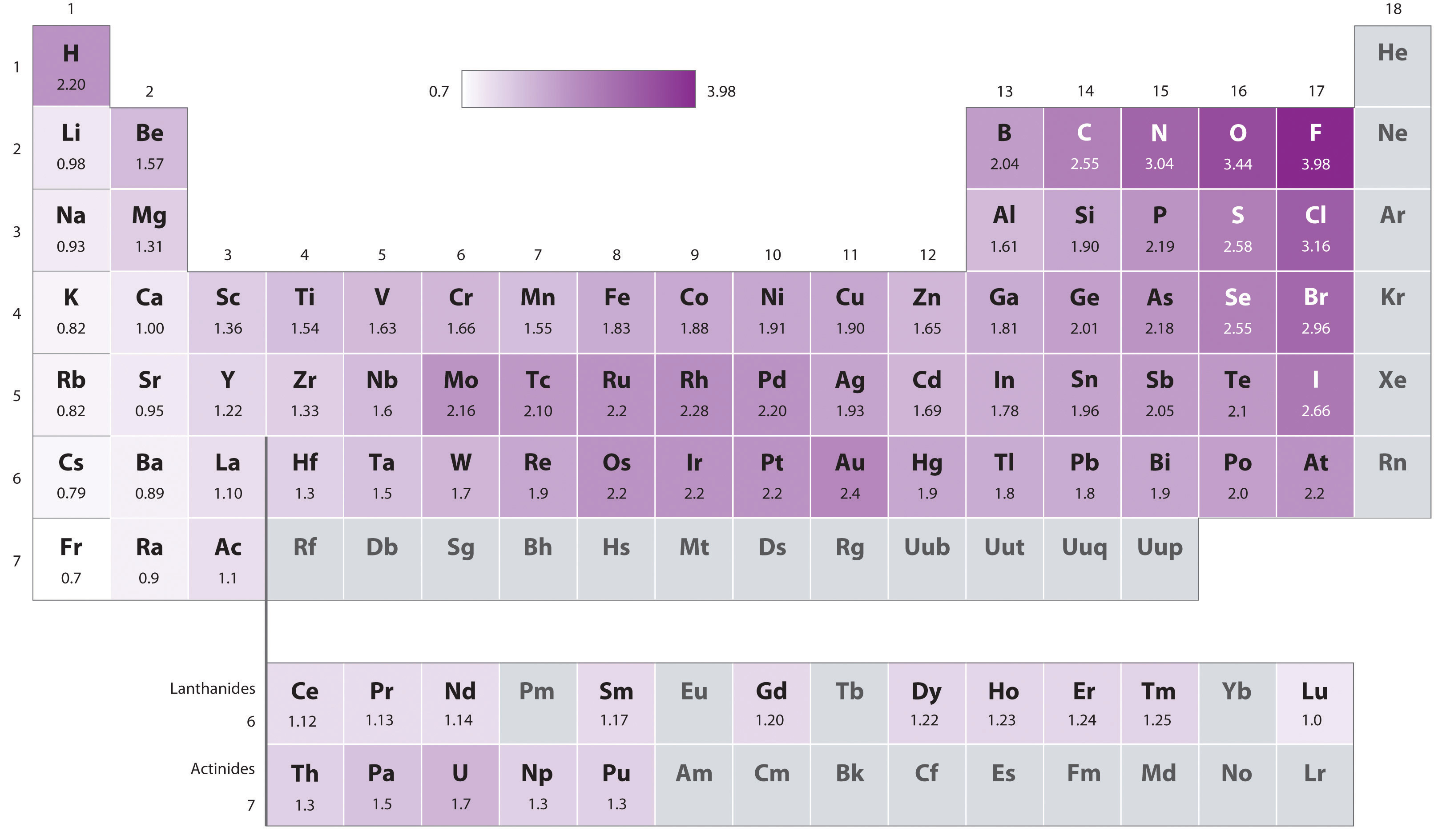
Table \(\PageIndex{1}\): Paulings scale of electron affinities of the elements. When a bond forms between two elements, the more electronegative element has a stronger pull for electrons than the more electropositive element.

Exercise \(\PageIndex{1}\)

Why do the Noble Gases in Table 8.7.1 not have a value for electronegativity?

Answer:

Remember, electronegativity is not a thermodynamic property, but a relative value given to an atom in a bond, which indicates how strongly it pulls the shared electron density towards itself. The noble gasses tend to not bond with other elements, which is why we call them noble, and thus it does not make sense to give them a value.

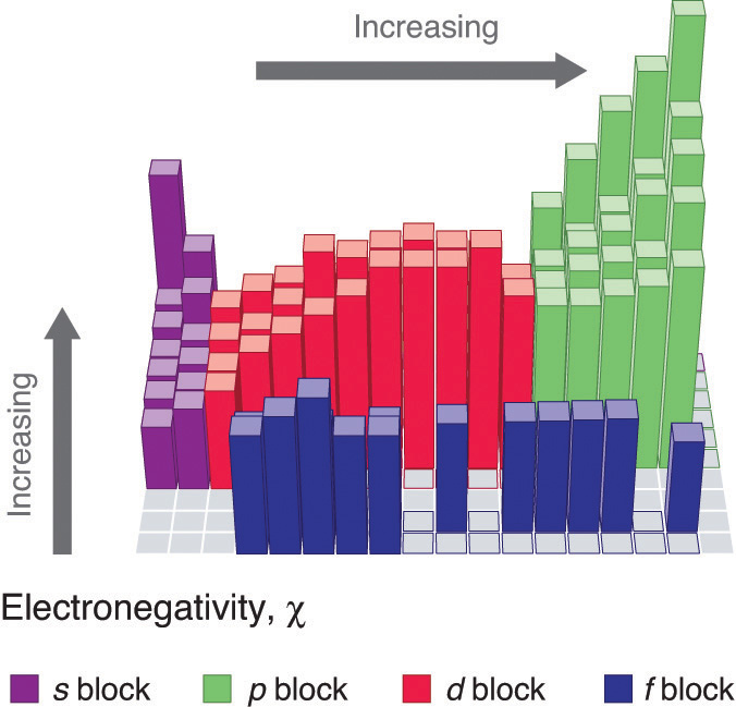
Figure \(\PageIndex{2}\): Diagram showing periodic trends in electronegativity. Note going up a group and across a period results in an increase in electronegativity.

Exercise \(\PageIndex{2}\)

Why would going across (left to right) a period result in an increase in electronegativity?

Answer:

Remember that the effective nuclear charge increases going across a period, and the size of the atoms get smaller. This means the pull on the electron would be stronger, and so the trend makes sense.

Why would going down a group result in increased electropositivity (decreased electronegativity).

Answer:

Each element has an isoelectronic valence shell electron configuration, with the principle quantum number getting larger, meaning the valence electrons are farther away from the nucleus. This means they are less tightly held and so it would be less electronegative.

Without a table of electronegativities, would you be expected to know which would be greater

a). Mercury or Silver?
b). Mercury of Indium?

Answer:

a) No, as going up the periodic table increases \(\chi\) while going right to left decreases it. That is, (\(\chi\)-{Cd}>(\(\chi\)-{Hg} while (\(\chi\)-{Ag}<(\(\chi\)-{Cd}, and you do not know which effect is the greater. (The trends oppose each other.)

b) Yes, as going up and left to right both increase \(\chi\), (\(\chi\)-{Cd}>(\(\chi\)-{Hg} but going right to left decreases, (\(\chi\)-{In}>(\(\chi\)-{Cd}, so In must be greater than Hg

Rule of Thumb: Predicting Bond Types

As a "rule of thumb", electronegativity differences can be used to predict if a bond will be covalent, polar covalent or ionic. If the difference in \(\chi\) between two bonding atoms is less than 1/2, they are of very similar electronegativity and it is a covalent bond. If it is greater than 2 they are substantially different and more electronegative atom completely removes a valence electron from the electropositive, forming an ionic compound, and if it is between 0.5 and 2.0 it is polar covalent.

Difference in Electronegativity (\(\chi\))	Bond Type	Example
<0.5	Covalent	Cl-Cl (\(\Delta \chi\)=0), C-H (\(\Delta \chi\)=0.35)
0.5-2.0	Polar Covalent	H-Cl (\(\Delta \chi\)=0.96)
>2.0	Ionic	Na-Cl (\(\Delta \chi\)=2.23)

Table \(\PageIndex{2}\):

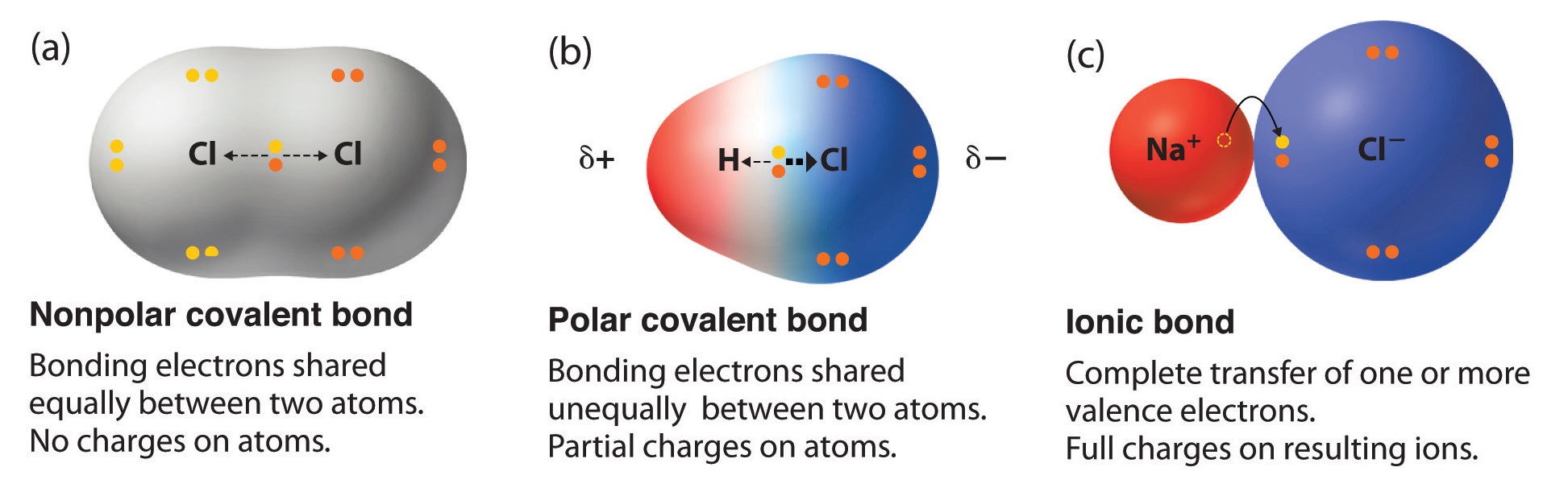
Figure \(\PageIndex{3}\): Illustration of different bond types between atoms of different electronegativities (see table 8.7.1 for \(\chi\) values and table 8.7.2 for (\(\Delta \chi\) values).

YouTube Videos on Electronegativity

Animated YouTube going over electronegativity and bond types

1:26 min YouTube uploaded by dkosasihiskandarsjah.

Note

2:11 minute YouTube going over electronegativity by RicochetScience

Dipole Moments of Diatomics

If the difference in electronegativity between the atoms of a bond are between 0.5 and 2.0 we can determine that the bond is polar, and if the atom is a diatomic, that must result in a polar molecule.

\[ \begin{matrix}
_{\delta ^{+}}& & _{\delta ^{-}}\\
H\; \; &-& Cl
\end{matrix} \]

Polar molecules have a positive and negative end, which will align with an external electric field as shown in figure 8.7.4

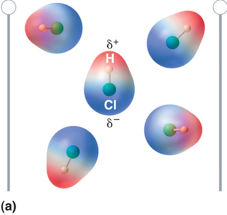
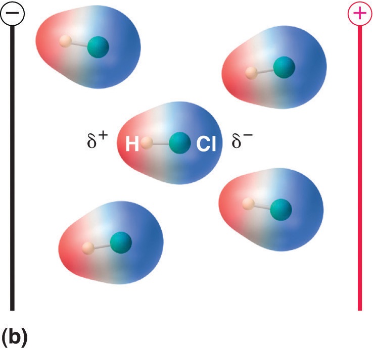
Figure \(\PageIndex{4}\): Consider gaseous HCl where there is no interaction between the HCl molecules. In that absence of an external electric field (a) the molecules have random orientation, in the presence of an electric field (b) they align with the field as the \(\delta ^{+}\) end of the polar molecule is attracted towards the negative plate of the external field and the \(\delta ^{-}\) end is attracted towards the positive plate of the external field. Since the molecule is being pulled in opposite directions it does no migrate to the field the way an ion would, but aligns with the field.

Dipole Moment

An electric dipole occurs when two equal charges are separated by a distance. The dipole moment is a vector \(\vec{\mu}\), which is a measure of the electric dipole's strength and orientation and has the units of the Debye. The dipole moment of a molecule is a function of the partial charges of the polar bond, and the distance between them. Ignoring the vector aspects, this can be calculated by Equation:

\[\mu = qr\]

where

• \(\mu\) is the dipole moment (really a vector)
• q is the magnitude of the partial charges \(q^+\) or \(q^-\) (or the more commonly used terms \(δ^+\) and \(δ^-\)), and
• r is the distance between the two charges of the dipole moment (which is also a vector).

The Debye is a very small unit, which in terms of SI base units has a value of 3.34x10^-30 Amp meter seconds. Note, Yocto, (10^-24) is the smallest SI prefix and this is of the order of 10⁶ times smaller!

Relating Dipole Moments to \(\Delta \chi\) and bond lengths:

In table 8.7.2 we look at the diatomic molecules between H and the halogens. We note that as you go down the periodic table the bond length increases, which would result in a large dipole moment. But it goes down because the \(\Delta \chi\) decreases to a greater extend. So the difference in electronegativity is the major factor in determining the strength of the polarity of a molecule..

Table \(\PageIndex{2}\): Relationship between Bond length, Electronegativity and Dipole moments in simple Diatomics

Compound	Bond Length (Å)	Electronegativity Difference	Dipole Moment (D)
HF	0.92	1.9	1.82
HCl	1.27	0.9	1.08
HBr	1.41	0.7	0.82
HI	1.61	0.4	0.44

Note:

In this class you will not be performing calculations with \(\mu\), but you do need a conceptual understanding, and you need to understand the difference between the charge of an ion, and the magnitude of the dipole moment of a polar molecule. So far we have kept to simple diatomics. In the next section we will move onto compounds with more than one polar bond, and see that the orientation of the bonds affects the polarity of a molecule, and that a symmetric molecule like carbon dioxide has polar bonds, but is in itself, nonpolar.