10.5 Kinetic Molecular Theory of Gases

Template:Chem1402Belford

Introduction

The Kinetic Molecular Theory (KMT) describes an Ideal Gas, PV=nRT.

The laws that we have discussed so far are empirical laws, in that they were derived from experimental measurements. The kinetic molecular theory is based on fundamental principles that explain the behavior of a gas that follows the ideal gas law. There are five postulates to the Kinetic Molecular Theory, and gases will deviate from the ideal gas law when theses postulates break down.

Five Postulates of KMT.

1. Gas particles travel in straight lines unless they collide with other particles or the walls of the container.
2. Gas particles have negligible volume compared to the free space between them..
3. Molecular collisions are perfectly elastic and kinetic energy is conserved.
4. Gas particles experience negligible intermolecular forces, there are no attractive or repulsive forces between particles.
5. The average kinetic energy of the particles in a sample of gas is proportional to the temperature.

Kinetic Molecular Theory (KMT) and Gas Laws

Before proceeding we should look at figure 10.5.1 and realize that although one can describe a particle as being in the gas phase, a gas is not a particle, but a very large number of particles if they are to be empirically measured, and they are an ideal gas is the follow the postulates of Kinetic Molecular Theory (KMT). This is exemplified by the eq. 10.5.1, which shows that in an easily measurable quantity like one liter, there are more than 10²⁴ particles of Xenon gas .

How many particles of Xenon are in 1.00 liter at STP?
STP is 1 bar (0.98592 atm) at 273.15K, which is the freezing point of water, and we know that the molar volume of any ideal gas is 22.4L. So:
\[1.00L(\frac{1molXe}{22.4L})(\frac{131.3gXe}{mol})\frac{6.022x10^{23}atoms}{mol}=3.53x10^{24}atoms\; Xe\]

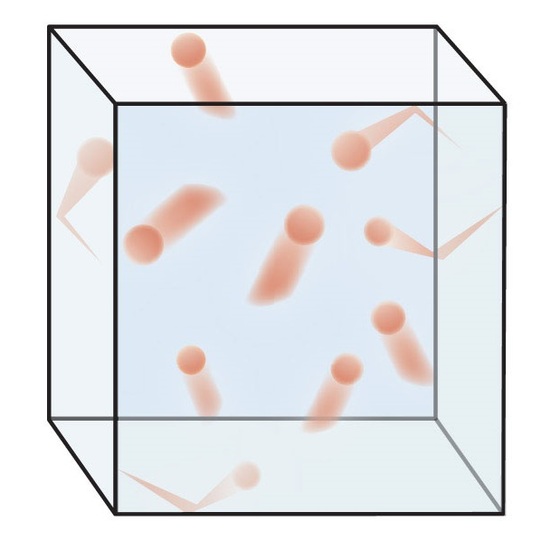
As such, the two images of figure 10.5.1 are very useful in understanding an ideal gas. The image on the left represents a gas phase system of many molecules moving in linear motion and undergoing elastic collisions with the surface. By using a cube it is easy to describe this system in terms of Cartesian coordinates, where there are 6 faces, two along each axis. It also needs to be understood that velocity is a vector, which has a magnitude and a direction (speed is a scalar and only has magnitude). There are two implications to this. First, each particle of gas can have a component of its velocity that represents translation along each of the Cartesian axis (v_x, v_y​​​​​ & v_z) and second, that translation can be in either the positive or negative direction.

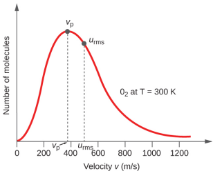Fig. 10.5.1(a)Gas molecules moving in different directions with different velocities	(b) "Velocity profile" representing a large number of gas molecules, vp is the most probable velocity and urms is the root mean square speed (average velocity). Note, these are actually speeds (a scalar) because velocity includes direction.

Part (b) of figure 10.5.1 is a velocity profile and is worth taking a moment to become familiar with. The area under the curve represents a molecular system, which would be 3.53 x 10²⁴ atoms if we were discussing 1 liter of Xe gas at STP. We note that kinetic energy for translational motion is 1/2mv², (m = mass, v= velocity), and at any point in time some molecules are moving very fast (high kinetic energy), while others are moving slow (low kinetic energy). The peak of the curve represents the most probable velocity (the velocity the greatest number of molecules have) and if the curve is symmetric, this is also the average velocity. Usually though, the curve is asymmetric, with a tail into the high velocity region as indicated here, and we indicate the average velocity as the room mean square speed (u_rms)

Average root mean square speed for a system of n particles with individual velocities u_i:
\[u_\ce{rms}=\sqrt{\overline{u^2}}=\sqrt{\dfrac{u^2_1+u^2_2+u^2_3+u^2_4+…}{n}}\]

Why do we use root mean square speed and not the arithmetic average velocity

Remember velocity is a vector, and something can be moving along either the [+] or [-] directions of an axis, and for a large system of particles in random motion the number moving in the [+] or [-] is directions are roughly the same. The sum of a symmetric distribution of speeds and directions would be zero. By squaring each individual velocity all values become [+], allowing summation without cancelation, and then dividing by the total number of particles gives the average velocity square. The square root is taken to remove the effect of squaring, but the resulting value is a speed (scalar) as it has a magnitude, but no direction (vector). The important take-home message of figure 10.5.1 is that a gas is a system of particles, each particle of which has a unique location, velocity and kinetic energy, and that we use the average kinetic energy to define the system (even though most of the particles actually have a different energy).

\[\mathrm{KE_{avg}}=\dfrac{1}{2}mu^2_\ce{rms}\]

Boyle's Law & KMT (const. n,T)

At constant n and T, the velocity profile on part (b) of figure 10.5.1 stays the same. Here we are looking at closed (constant n) isothermal (constant T) elastic system that has no resistance or heat loss to expansion or contraction.

a. Effect of \(\Delta V \) on P:
Reducing the volume of the cube in part (a) of figure 10.5.1 increases the pressure because it increases the collision frequency of the particles with the wall. This is because they are maintaining the same velocity but have less distance to travel as they traverse the cube. Likewise, Increasing Volume decreases pressure beacuse it takes longer to traverse the expanded cube, resulting in a reduction in the collision frequency. Remember Pressure is force per unit area, and the force is the consequence of the change in momentum of the gas particle as it undergoes an elastic collision with the wall of the container (this is called an impulse in physics).

b. Effect of \(\Delta P\) on V:

Figure 10.5.2 shows this effect. Here we have a cylinder type system with a gas in a closed system. If the internal pressure is not equal to the external, the system will adjust until the are equal. Consider a system starting at state (b) where the internal volume is 3 dm³ and the pressure is 1.97 atm. If you then reduced the external pressure to 0.987 atm, the force/unit ares inside is greater than outside and the system expands until they balance and equilibrium is re-established (a). Note, in this case we cut the pressure in half, and so the volume doubled.

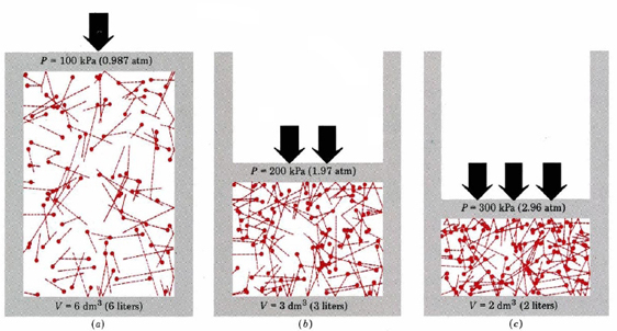
Fig. 10.5.2: Relationship between P and V, note, these conditions are equilibrium conditions.

On the other hand, we could have increased the pressure of the system at (b) to 2.96 atm and now the external pressure is greater and so the system contracts until a new equilibrium is acheived (c). KMT accounts for these effects because the particles are seen to travel in straight lines until they collide with the walls of the container. Since T and n are constant, the relationship is defined by the length of the path the particles travel as they traverse the container. A larger free path (bigger V) means they collide less with the wall and so P goes down. A smaller free path means the collide with the wall more frequently, and so P goes up.

Charles Law (constant n,P)

This describes a closed elastic isobaric system that can freely expand and contract. Figure 10.5.3 shows how heating a system affects the velocity profile. Note, since n (number of molecules) is constant the area under each curve is the same. At higher temperatures the curves flatten out and move to the right, increasing u_rms and thus the average kinetic energy. This has two effects, first, collision frequency goes up because the the faster moving particles traverse the container quicker, and second, each collision has more energy because the particle is moving faster (E_K=1/2mv²). Since the pressure (force per unit area) is being maintained constant, the area must go up to offset the increased force, and so the container expands as T goes up.

Fig. 10.5.3 Velocity profiles of Nitrogen at different temperatures. Note that even at high temperatures some of the molecules have low velocities, but as T goes up, u_rms goes up.

Can you cool the curve to absolute zero?

No, at some point you reach the boiling point and cooling below that causes the system to convert to a liquid, and you no longer have a gas.

Avogadro's Law (const P,T)

This describes an elastic container at isobaric and isothermal conditions. According to KMT increasing the number of particles increases the collision frequency on the surface which effectively increases the force. Since pressure (force per unit area) is constant, the system must expand (increase surface area) to accommodate the increased number of collisions.

Annimation 10.5.1: Change the number of moleculesChanging the number of molecules and click the start button. Note how adding molecules increases the collision frequency. Since pressure is being kept equal, the system adjusts its volume so the collision frequency returns to the original value.

KMT and Ideal Gas Law

Qualitatively,KMT predicts:

1. More particles means more collisions with the wall (P \(\propto n\))
2. Smaller volume means more frequent collisions with the wall (\(P\propto\frac{1}{V}\))
3. Higher molecular speeds means more frequent collisions with the walls (P \(\propto T\))

Putting all of these together yields

\[ P \propto \dfrac{nT}{V} =k \dfrac{nT}{V}\]

which can be rewritten as the familiar Ideal gas equation:
\[ PV=nRT\]

It can be shown that the kinetic energy of a gas that is free to move in one direction is KE = 1/2nRT, and a gas that can move in three dimensions is 3/2nRT.

This allows us to relate the average root mean square velocity to the molar mass of a molecule.

\[ PV=\frac{3}{2}nRT=N_{T}(\frac{1}{2}m_{A}u_{rms}^{2})\]

Where N_T = total number of gas molecules and m_A = mass of an individual atom (amu).

Noting the number of moles is the total number of molecules (N) divided by Avogadro's number (N_A = 6.022x10²³).

Ignoring the first (PV) part we can cancel the 1/2 and substitute for N_T: N_T = nN_A

\[3nRT=n(N_{A}m_{A})u_{rms}^{2}\]

noting \(\mathfrak{M}=N_{A}m_{A},\; \;where \; \mathfrak{M}=molar \;mass\) and cancelling n gives

\[3RT=\mathfrak{M}_{A}u_{rms}^{2}\]

or

\[ u_{rms}=\sqrt{\frac{3RT}{\mathfrak{M}}}\]