2.1: Introduction to Python

Python

Python is an open source object-oriented programming language. It is interpreted in contrast to compiled, which means you can write some code and run it from the command line or an appropriate editor, and the program compiles the line of script you run into to machine readable language as you execute the code, without your having to convert the entire cscriot to machine readable code. In a compiled program, the computer is giving the entire script as machine readable code from the get go.  The advantage of a compiled program is that it is "closer" to the operating system and so you can control things at a very granular level, like how much memory is allocated to a task. 

We will run Python scripts in two different ways.

• From the command line
• From and an Integrated Development Environment (IDE)

Raspberry Pi (RPi) uses Linux as an operating system and Bash is the default interpreter, and we will also have lessons on both Bash scripts. We will develop Python code in the Thonny IDE that you will install in the next section of this lesson plan. We are choosing to use Thonny as it is also installed on your RPi, and so you can write code on your personal computer and then then transfer it to the RPi (or vice versa). A Python interpreter is also bundled into the Thonny installation and so after you instal Thonny you can instantly start writing Python code

Python is only part of the IOST ecosystem and there are many other programs that you will want to use as you advance in your studies of digital sciences. After you install Thonny we will a second version of Python using the miniconda version of the Anaconda data science platform (see below). We will then redirect Thonny to use the miniconda python interpreter in contrast to the default version.  This will not only allow you to add additional dat science packages but assist you in updating and maintaining your Python installation.

Thonny

If you choose to use Thonny go to  https://thonny.org and install the software apropriate for your operating system.  As of January 2022 this will be version 3.3.12 and it will also instal Python 3.7.  If you need help, this Youtube video quickly goes over the process (https://youtu.be/TlvQOWhlfpo).

 

UI Modes

Thonny has three UI (User Interface) modes, Simple, Regular and Expert.  We will typically use the Simple or Regular mode.  On your PC you will probably want Regular as it has access to the file menu (fig. \(\PageIndex{2}\)), but if you have limited screen space, like are on a Pi with a low resolution monitor, you may wish to use simple mode to maximize the screen's realestate.

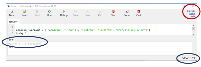Figure \(\PageIndex{1}\): Thonny UI in SIMPLE MODE, note there is no menu bar (see image below).  (Copyright; Belford, CC 0.0)

To switch to REGULAR mode you can click the text in the circle of the upper right in figure \(\PageIndex{1}\). To switch from regular mode to simplemode go to tools/options/general/UI mode and pick the option you want (figure \(\PageIndex{2}\)).  Also, note that the blue oblong circle on the shell of figure \(\PageIndex{1}\) shows that Thonny is running python 3.7.9, which was co-installed with Thonny, but in \(\PageIndex{2}\) we can see that Python 3.9.7 is being run. That is, these images were taken when we were using different versions of Python, and in the next section you will install Python 

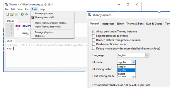Figure \(\PageIndex{2}\): Thonny UI in regular mode.(Copyright; Belford, CC 0.0)

To switch from regular mode to simple mode  choose Tools/General/UI mode/regular (Figure \(\PageIndex{2}\)). We will typically use the Regular mode.

Menu Items

When in Regular mode you have access to several menu items and it is prudent to go over these before starting.  Many of these like open and save will be familiar to you while others will be unfamiliar.  It is always a good idea to check out menu items on any software package before you start using it.

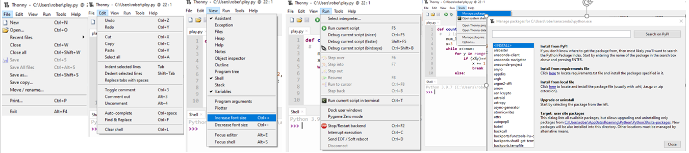Figure \(\PageIndex{3}\): Copy and Paste Caption here. (Copyright; author via source)

 

We will take a quick dive on several of the menu item features that your are probably not familiar with.

Edit

In some IDEs you need to save a file before you run it.  In Thonny you do not, and the moment you hit "RUN" it saves the file and then runs it.  This means it overwrites the code of the original file. So, a common error is to change some code and run it to see if it works, but you then lose the original code.  A good practice is to comment out code with the # symbol.  This means that text will not be operated on.  In the Edit menu you have the ability to comment or uncomment large blocks.

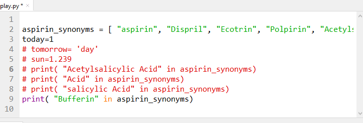Figure \(\PageIndex{4}\): By clicking comment out in the Edit menu we were able to prevent lines 4-8 from being run. We could then try some other script, and if it did not work, we could simple uncomment these in the Edit menu, and not lose the code. It is very important to realize that in Thonny saves code the moment you run it, so if you edit something and run it, you lose the original code. (Copyright; Belford CC 0.0)

Note, the color coding above is a result of the option chosen in the tools/options/theme-fonts tab.

View

The View option allows you to select the interfaces you wish to work with. The code editor is always present and you probably want to run the Shell, which emulates a command line interface. In figure (\(\PageIndex{3}\)) the Shell, Variables and Assistant options have been opened. We will go over the utility of these features as the course proceeds, but these are probably the most common ones you will wish to work with.

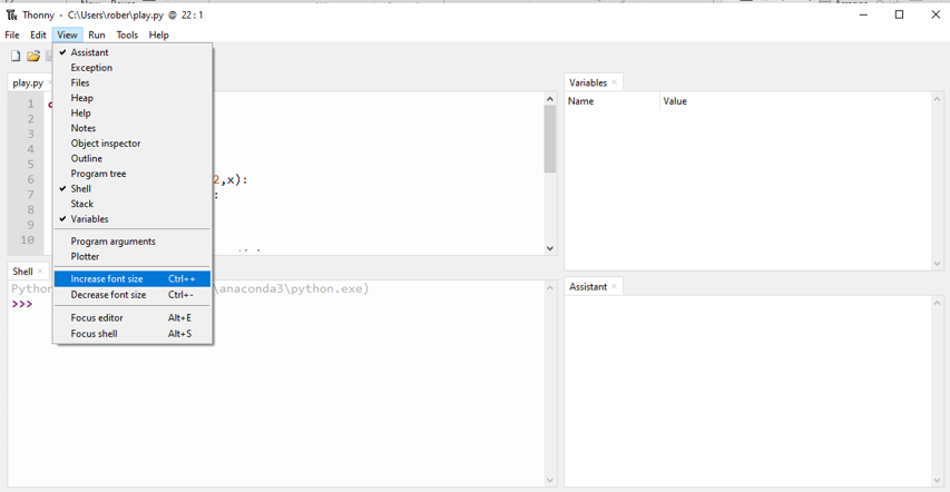Figure \(\PageIndex{3}\): View menu options for Thonny UI. (Copyright; Belford, CC 0.0)

You will also note that the View menu provides an option to increase or decrease font size with keyboard shortcuts of Ctrl + + and Ctrl + - (click the crtl followed by either plus or minus).  This is often very important when you are running a Pi in headless mode using the VNC viewer.

Run

The run tab allows you to execute python code in the editor and interact with it through the shell. You will often want to use the <F5> shortcut key.  You can also run the program in "debugger mode" that allows you to walk through the code one step at a time.  There are a lot of YouTube videos on the debugger and the following one goes over it (we are starting where the debugger part of the script is, but you may want to watch the entire video.

 

 

Tools

Tools is an important menu item, in fact we have already looked at in in figure \(\PageIndex{2}\) when we switched the UI (User Interface) from simple to regular mode. Let's quickly look at some of the other features of the Tools, starting with the manage packages and manage plugins.  A Python package is a way to add new features to your program, like say math or time functions, and is essentially a directory of modules that you typically download from a service like the PyPI Python Package Index, that as of 1/22/2022 contains 351,947 projects. A package has a init_.py file sets how the packages are imported, while a directory could be a collection of python modules, but without the init_.py file, they will not be integrated into the interpreter.

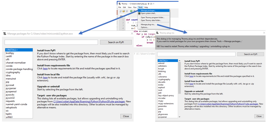Figure \(\PageIndex{6}\): If you are running the default python interpeter that comes with Thonny you can manage packages from this menu.  If you are using a different interpreter, say the one from Anaconda (see below), you would not use this option.  The manage packages allows you to install new packages while the manage plug-ins is used for managing existing plug-ins. . (Copyright; Bob Belford, CC 0.0)

We have already looked at the options submenu when we changed the UI (Figure \(\PageIndex{2}\).

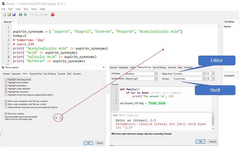Figure \(\PageIndex{7}\): Editor and "Theme & Font" submenu items of the "options" item of tools overlaid on the IDE. (Copyright; Belford CC 0.0)

PEP 8, the Index of Python Enhancement Proposal style guide suggests a maximum line length of 79 characters and you can set a verticle line in your editor to warn you when your string of code is getting to long (figure \(\PageIndex{7}\)).

 

Anaconda

Anaconda is a data science platform which allows you to find and install over 7,500 data science and machine learning package and progarams like Python, R, Jupyter, Scikit learn, matplotlib and R, but also includes the conda package manager that helps deal with conflicts across software.  There are two installation options, Anaconda and Miniconda. If you are planning to get involved with Data Sciences or have a high quality computer you will probably want to install the full version of Anaconda, but if this class is your only endeavor than you will probably want to install the Miniconda version.  Note, the full version comes the Anaconda Navigator which makes it very easy to launch and maintaint packages, where the Miniconda requires you to use to launch programs through the conda prompt.  What we are going to do in this class is connect the Thonny IDE to the Python interpreter installed with either Anaconda or Miniconda and use Thonny to launch Python.  We are choosing Thonny because it comes installed with the Raspberry Pi.

• Anaconda
  • https://www.anaconda.com/
    • Well suited for scientific programmings.  Comes with ipython and Spyder, and the Conda package management system.
    • Has 1500 scientific packages and uses 3GB of disk space
• Miniconda
  • https://docs.conda.io/en/latest/miniconda.html
  • Anaconda without all the packages

You are welcome to use the default python interpreter with Thonny of instal it through Anaonda. Figure \(\(PageIndex{8}\) has screen shots for using miniconda.

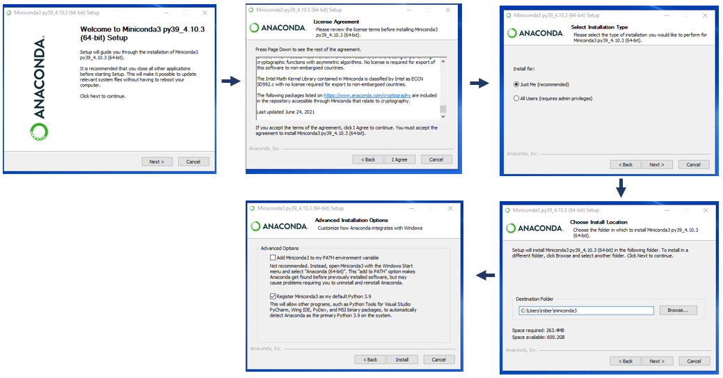Figure \(\PageIndex{8}\):Screen captures of steps involved with installing miniconda. (Copyright; Bob Belford, CC 0.0)

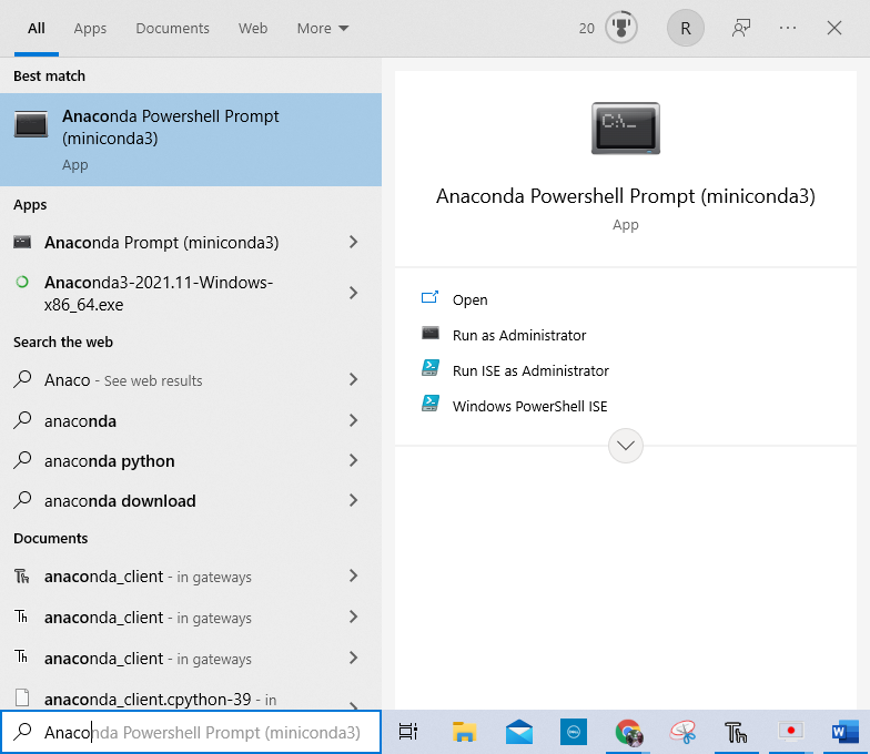
Once you install miniconda you want to open the Anaconda prompt (miniconda 3) from your Windows start menu, which can be done by typing in the search

 

Figure \(\PageIndex{9}\): Opening the Anaconda command prompt for miniconda in Windows 10. (Copyright; Belford CCC 0.0)

to update your packages you want to type the following into the command prompt.  You first need to navigate to the correct folder.  In the command prompt (which is a terminal shell) type ls to see your folders.

Note <cctrl> C bring back the command prompt if you get stuck

ls

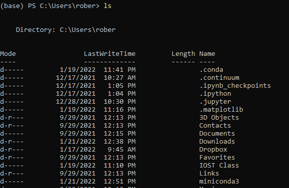Figure \(\PageIndex{10}\): Viewing directory to locate where conda is installed. (Copyright; author via source)

Now move to that directory (Change Directory) 

 cd .\miniconda3\

When you list the files you will see where you installed python

You will also want to update python

conda update python

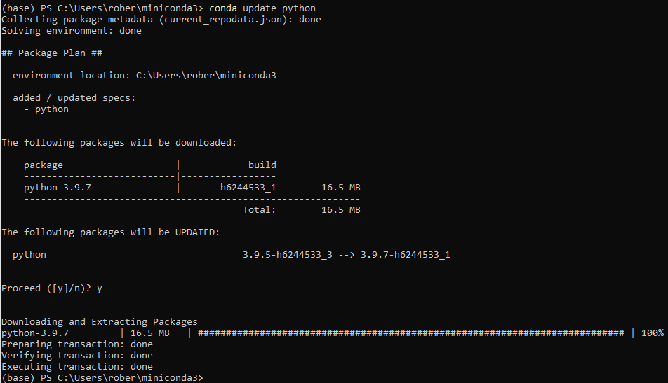Figure \(\PageIndex{11}\): Screen shot showing how to update python with miniconda. (Copyright; Belford CC 0.0)

Exit the anaconda shell

exit

Now we want to link our Thonny to the new install of python.  Open Thonny and go to tools/options/interpreter (figure \(\PageIndex{12}\)) and choose the "Alternative Python 3 interpreter or virtual environment".  Initially the python executable will direct to where you installed Thonny and you need to direct it to the new path, which you found above.  Or you can click the three dots tothe right of the current path and navigate to where the python application file is located and open it.

 

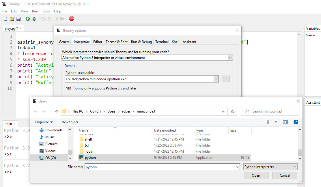
Figure \(\PageIndex{12}\): Copy and Paste Caption here. (Copyright; author via source)

If you now look at the shell in Thonny you can see the new updated Python program you are running

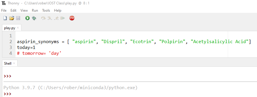Figure \(\PageIndex{13}\): the version and path of the Python Interpreter Thonny is using. (Copyright; Belford CC 0.0)