8.4: Data Analysis

Data Analysis:

 

Overview

Figure \(\PageIndex{8}\) shows the features of the Job's plot analysis you will develop with your Google Workbook.  For a bidentate ligand we expect three possible formulas; ML₃ (red line at x_m=0.25), ML₂ (purple line at x_m= 0.33) and ML (green line at x_m= 0.50). You will plot three series of data in your sheet.  Series A is all the data.  Series B (in red) is the data where the ligand is in excess and drives the metal to be completely consumed. Series C (in yellow) is where the metal is in excess and drives the ligand to be completely consumed. If there was no equilibria and all the reactants convert to products these two trend lines would cross when the reagents are in stoichiometric proportions. From the graph this occurs closest to the mole fractions associated with ML₃., and so we will consider this to occur at m_x = 0.25.  It is clear that as the proportions approach stoichiometric proportions the real curve (blue dots) deviate from the straight line functions where a reagent was in excess and this is due to the fact the an equilibria exists between coordination complex and the metal and ligands.

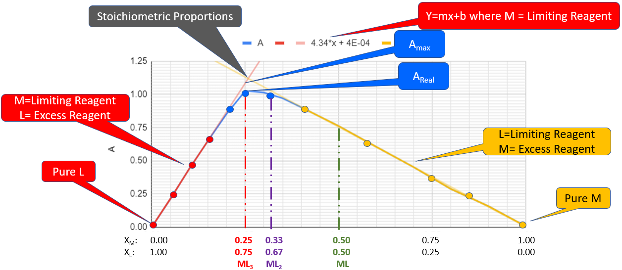Figure \(\PageIndex{8}\): Jobs plot within the Google Workbook.  Note there are three concentrations where the reactants could be in stoichiometric proportions.  ML₃ (red at X_m=0.25),  ML₂ (purple at X_m=0.33) and ML (green at X_m=0.50). In this graph the trend lines from the regions where one reagent was in excess cross at around 0.27, so we will consider the formula to be ML₃ and the complex forms at x_m=0.25 and c_L=0.75 (Copyright; Bob Belford & Liliane Poirot CC-BY)

A_real

A_real is the absorbance of the solution taken from the data sheet when they are in stoichiometric proportions.  for figure \(\PageIndex{8}\) this was 1.027 (the data is not shown, but use the value of your data sheet when they are in stoichiometric proportions)

A_max

A_max is the value of the absorbance if the theoretical yield was 100%. This can be calculated by using the equation for the straight line in the excess ligand region and calculating the value of A at xm=0.25.  That is, when there was excess ligand it essentially used up all the limiting reagent as the system achieved equilibrium.

\[A_{max}=4.34(0.25) + 0.0004 = 1.085\]

C_max

C_max is based on 100% theoretical yield when the reactants are in stoichiometric proportions (where the two trend lines intersect).  For figure \(\PageIndex{9}\) this occurs as x_m= 0.25 and if the initial ferrous iron concentrtation was 0.005M, the complex ion concentration [FeL₃⁺²] is:

\[0.25(.005M)= 0.00125M\]

C_real

To calculate K_f we need to know the concentration of the coordination complex and this can be done by applying the two state approach to Beer's Law (A=\(\epsilon bc\)) and simplifying.  It should be noted the C represents the complex ion concentration ([ML_b]⁺² for a complex with b ligands.

\[\frac{A_1}{A_2} =\frac{\epsilon bC_1}{\epsilon bC_2} \\ \; \\ so \\ \; \\ \frac{A_1}{A_2} =\frac{C_1}{C_2}\]

So if state "1" is the real concentration and state "2" is the hypothetical "max" concentration if there was 100% theoretical yield, we get

\[C_{real}=C_{max}\frac{A_{real}}{A_{max}}\]

Based on the above data, \[C_{real}=0.00125M\left ( \frac{1.027}{1.085} \right )=0.00118M\]

Calculating K_f

Figure \(\PageIndex{9}\) represents the formation of the complex ML because the peak is when the mole fraction of M and L are both 0.5.  If we look at the complex MLb where "b" is the number of ligands we have three possible equilbrium constants and the following generic RICE diagram.

\[M + L \rightleftharpoons ML \;\;\left ( K_f=\frac{[ML]}{[M][L]} \right ) \\ \; \\ M + 2L \rightleftharpoons ML_2 \;\; \;\;\left ( K_f=\frac{[ML_2]}{[M][L]^2} \right ) \\ \;\\ M + 3L \rightleftharpoons ML_3 \;\;\;\;\left ( K_f=\frac{[ML_3]}{[M][L]^3} \right )\]

Reactants	M	+	bL	⇌	MLb
Initial	[M]Initial		[L]Initial		0
Change	-x		-bx		+x
Equilibrium	[M]Eq=[M]Initial-x		[L]Eq=[L]Initial-bx		[MLb]Eq=x

 

Noting C_REAL is ML_b because it is the complex ion that is absorbing the light.  So we know know the extent of reaction (x), and can solve for the equilibrium concentration of all species using the K_f expression appropriate to the complex ion being formed (b=1, 2 or 3).

\[K=\frac{x}{(M_i-x)(L_i-bx)^b}\]

For the above example where x_m=0.25 we have the formula of ML₃ and when at stoichiometric proportions ML₃= C_real=0.00118M

Reactants	M	+	bL	⇌	MLb
Initial	.25(.005)=[0.00125]		0.75(.005)=[.00375]		0
Change	-0.00118		-3(0.00118)		+0.00118
Equilibrium	0.00007		0.00021		0.00118

\[K_f=\frac{0.00118}{0.00007\left ( 0.00021 \right )^3}=1.82x10^{12}\]

Cover Page

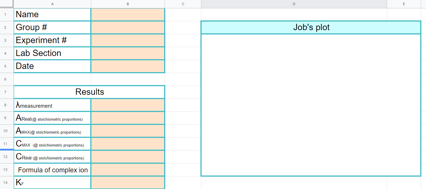
Figure \(\PageIndex{9}\): Note  C_max is the concentration of the complex ion based on the theoretical yield and C_real is the actual concentration of the complex ion due to an equilibria between reactants and products.   (Copyright; Bob Belford & Liliane Poirot CC.0)

Note, for the formula use ML, ML₂ or ML₃.  (you can make the font size of the numbers smaller so it looks like a subscript)

Data Sheet

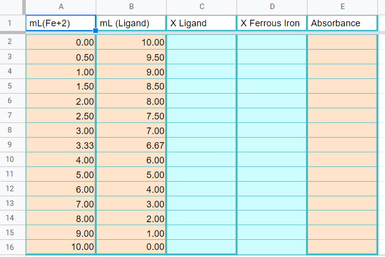Figure \(\PageIndex{10}\): Copy the data from the data sheet handout to this page in your workbook.  Be sure to copy the wavelength you measured the absorbance at on the title page (Copyright; Bob Belford & Liliane Poirot, CC0)

 

Job's Plot

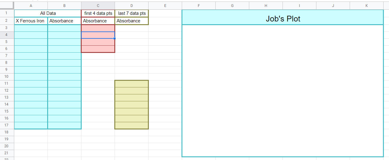Figure \(\PageIndex{11}\): When completed this graph will have three series of data. The first is a scatter plot of all the data. The second is a trend line with equation of the first 4 datapoints (column C) and the last is the trendline of the last 7 data points (column D).  Where the trendlines intersect will be used to determine the stoichiometric proportions of the metal and ligand as they form the complex ion (Copyright; Bob Belford & Liliane Poirot CC.0)

 

1. Paste data into columns A and B using ctrl+shift+v
2. Copy first 4 absorbance data points

The following YouTube provides instructions for creating the Job's plot.

 

Rice Table

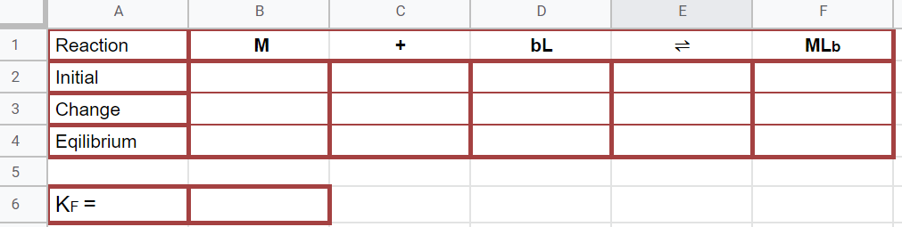Figure \(\PageIndex{12}\): Rice diagram for calculating the formation constant. (Copyright; Bob Belford & Liliane Poirot CC0.0)

The data for the RICE table represents the reactants when they are mixed in stoichiometric proportions.  The initial concentrations of the metal and ligand can be calculated from the mole fractions and the concentrations of the stock reagents mixed. The Equilibrium concentration [ML_b] is C_real.

 

 

 

 

 

 

 

Note

If there are more than one ligand there would be intermediates formed through a mechanism involving bimolecular collisions with the ligands and metal ions, or ligands and the intermediates. That is, there is a stepwise formation of the complex ion

\[M + L \rightleftharpoons ML \;\;\;(fast) \\ \; \\  ML + L \rightleftharpoons ML_2  \;\;\;(slower) \\ \;\\ ML_2 + L \rightleftharpoons ML_3  \;\;\;(slowest)\] 

When the metal is the limiting reagent and there is a lot of excess ligand (high X_L or low X_M), the theoretical yield based on the complete consumption of the limiting reagent (M) is achieved because of there is so little M that it all gets used up. Due to the excess [L] all of the equilibria are moved to the right and the final product is the major product.  When the ligand is the limiting reagent it is also consumed, but now there is a paucity of L and so many of the intermediates can exist in equilibrium. In fact at very low ligand mole fractions the intermediates are often the dominant product.  That is why in obtaining A_MAX we extrapolate from the side where metal is the limiting reagent, and not where L is.  If there were no intermediates (like in M + L ->ML) one could extrapolate back from the side of low ligand too, and where they meet would be the ratio of stoichiometric proportions (as in figure \(\PageIndex{9}\))

It should also be noted that the rates of the steps do not define the equilibrium constants, and that the formation constant of the final complex ion is often the largest.