3.9: Hybridized Orbital Energy Diagrams

Mixing Hybridized Orbitals and Formation of Antibonding orbitals

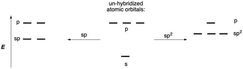
As shown in Section 3.4, the energy levels of hybridized atomic orbitals are a weighted average of the mixed atomic orbitals (Figure \(\PageIndex{1}\)). When two hybridized atoms approach each other, the orbitals mix to form bonds. However, as with hybridization, mixing of orbitals results in the exact same number of mixed orbitals as there were originally. This means that for every bonding orbital between atoms, there is an antibonding orbital, which is not shown in the diagrams in Chapter 3.4, for the sake of simplicity. Bonding orbitals are lower in energy than the starting atomic orbitals, and the corresponding antibonding orbitals are higher in energy. 

 

Figure \(\PageIndex{1}\): orbital energies of hybridized orbitals.

Bonding interactions with a large amount of spatial overlap will be the strongest (e.g., σ bonds) and those with less spatial overlap will be weaker (e.g., π bonds). Each interaction between hybridized orbitals will create an in-phase bonding interaction and an out-of-phase antibonding interaction. For more on bonding, antibonding, and phases of orbitals, see Chapter 3.2: Molecular Orbital Theory.

Hybridized orbital energy levels will vary based on the number of s and p orbitals that are hybridized. For example, sp hybridized orbitals have 50% "s-character" and 50% "p-character" and thus their energy will be halfway between the starting s and p orbital energies, and thus lower in energy than an sp² orbital on the same element (Figure \(\PageIndex{1}\)).

In the same way that we can use hybridized atoms to form bonds through overlapping hybridized orbitals in Chapter 3.4 and 3.5, we can form bonds between the orbitals using energy diagrams to gain insight into the energy levels of different bonds.

Example \(\PageIndex{1}\): Hybridized orbital energy diagram of ethane (C₂H₆)

Draw the hybridized orbital energy diagram of the C-C bond in ethane (C₂H₆). What is the lowest energy unoccupied orbital in this diagram?

Solution

1. The Lewis structure of ethane shows a single bond between the two carbons and single bonds with the six Hs.

2. The carbons in ethene are both sp3 hybridized, which gives us four sp³ orbitals. One of the hybridized orbitals on each carbon is involved in σ bonding (stronger interaction, lower energy bonding orbital). These two orbitals interact to form the bonding interaction, as well as an antibonding interaction. The remaining hybridized orbitals are involved in C-H bonds. There are no lone pairs or π bonds.

Example \(\PageIndex{1}\) shows how the starting hybridized atomic orbitals from Figure \(\PageIndex{1}\) mix to form bonding interactions and antibonding interactions in molecular orbitals. 

Example \(\PageIndex{2}\): Hybridized orbital energy diagram of ethene (C₂H₄)

Draw the hybridized orbital energy diagram of the C-C bond in ethene (C₂H₄). What is the lowest energy unoccupied orbital in this diagram?

Solution

1. The Lewis structure of ethene shows a double bond between the two carbons and single bonds with the four Hs.

2. The carbons in ethene are both sp² hybridized, which gives us one un-hybridized p orbital on each carbon atom and three sp² orbitals. One of the hybridized orbitals on each carbon is involved in σ bonding (stronger interaction, lower energy bonding orbital) and the un-hybridized p orbital on each carbon is involved in π bonding (weaker interaction). These interactions can be shown in the following diagram:

Example \(\PageIndex{2}\) shows how the starting hybridized atomic orbitals from Figure \(\PageIndex{1}\) mix to form bonding interactions and antibonding interactions in molecular orbitals. These molecular orbitals have different energies based on the overlap between the starting hybridized orbitals. The σ bond is formed between two sp² hybridized orbitals, which point towards each other, as shown in Chapter 3.5. This strong overlap in atomic orbitals results in a lower energy and more stable bonding orbital. The two p orbitals have less spatial overlap, and thus the bond is less strong between these atomic orbitals, and the corresponding bonding orbital is higher in energy. The stabilization gained in each bonding interaction is proportional to the destabilization of the antibonding orbitals.

 

Figure \(\PageIndex{2}\): In the ethene molecule, C₂H_4, there are (a) five σ bonds. One C–C σ bond results from overlap of sp² hybrid orbitals on the carbon atom with one sp² hybrid orbital on the other carbon atom. Four C–H bonds result from the overlap between the C atoms' sp² orbitals with s orbitals on the hydrogen atoms. (b) The π bond is formed by the side-by-side overlap of the two unhybridized p orbitals in the two carbon atoms. The two lobes of the π bond are above and below the plane of the σ system. Note: hybridized orbitals are shown as the major lobe to simplify the drawing.

 

Exercise \(\PageIndex{2}\)

Using hybridized orbital energy diagrams for bonding in HCN and H₂C=NH,

A) What are the hybridizations of each C and N?  

B) Which lone pair is highest in energy between these two molecules?

Answer

First, we need to draw the Lewis structures of each molecule, as shown below.

Then, we can assign their hybridizations based on the Lewis structures (Solution to A):

The hybridizations and Lewis structures will allow us to assign starting energies to the hybridized atomic orbitals:

Using these starting energies and the bonding shown in the Lewis structure, we can construct two hybridized orbital energy diagrams.

Now, using the hybridization of the N atoms in each diagram, we can see that an sp hybridized lone pair will be lower in energy than an sp² hybridized lone pair. Thus, the higher energy lone pair will be the lone pair in H₂C=NH.

Note 1: The nitrogen orbitals start lower in energy than the carbon orbitals, because N is more electronegative than C.

Note 2: The nitrogen orbitals are further apart than the carbon orbitals, because the s orbitals are more affected by electronegativity than p orbitals, which leads to a larger s/p orbital difference. 

Drawing Bonding and Antibonding Orbitals Starting with Hybridized Orbitals 

Figure \(\PageIndex{2}\) (above) shows a cartoon depiction of the bonding orbitals in ethene. These bonding orbitals are formed in the same way bonding orbitals in Molecular Orbital Diagrams are formed, through overlapping atomic orbitals. The corresponding antibonding orbitals can also be drawn in analogy to molecular orbitals (Chapter 3.2). 

Figure \(\PageIndex{3}\): bonding and antibonding orbitals formed with hybridized orbitals in ethene. 

The orbitals shown in Figure \(\PageIndex{3}\) have left and right lobes with the same "orbital density" because the left and right atoms have identical atomic orbitals. These orbitals will distort based on the electronegativities and atomic orbital energies of the starting orbitals - so bonds with two different elements or different hybridizations will have different shapes. 

Example \(\PageIndex{3}\): Drawing molecular orbitals with hybridized atoms with different electronegativities.

Draw the molecular orbitals (bonding and antibonding) corresponding to the C-N bond in HCN, using the solution to Exercise \(\PageIndex{2}\).

Solution

The orbitals we need to draw are the σ, σ*, π, and π*. Looking at the solution to Exercise \(\PageIndex{2}\), we can find that σ and π are closer in energy to N (more electronegative) and the σ* and π* are closer in energy to C. Thus, our bonding orbitals should be distorted toward N, and our antibonding orbitals will be distorted toward C. 

Example \(\PageIndex{3}\) shows how the molecular orbitals formed from hybridized atomic orbitals appear when distorted by atoms with different electronegativities. The p orbitals are combined to form two perpendicular π orbitals (in plane and out of plane) and two perpendicular π* orbitals. The σ and σ* orbitals are formed through the combination of sp hybridized orbitals, and are distorted by the difference in electronegativity between carbon and nitrogen.