
2: Determination of an Equilibrium Constant
- Page ID
- 204125
\( \newcommand{\vecs}[1]{\overset { \scriptstyle \rightharpoonup} {\mathbf{#1}} } \)
\( \newcommand{\vecd}[1]{\overset{-\!-\!\rightharpoonup}{\vphantom{a}\smash {#1}}} \)
\( \newcommand{\id}{\mathrm{id}}\) \( \newcommand{\Span}{\mathrm{span}}\)
( \newcommand{\kernel}{\mathrm{null}\,}\) \( \newcommand{\range}{\mathrm{range}\,}\)
\( \newcommand{\RealPart}{\mathrm{Re}}\) \( \newcommand{\ImaginaryPart}{\mathrm{Im}}\)
\( \newcommand{\Argument}{\mathrm{Arg}}\) \( \newcommand{\norm}[1]{\| #1 \|}\)
\( \newcommand{\inner}[2]{\langle #1, #2 \rangle}\)
\( \newcommand{\Span}{\mathrm{span}}\)
\( \newcommand{\id}{\mathrm{id}}\)
\( \newcommand{\Span}{\mathrm{span}}\)
\( \newcommand{\kernel}{\mathrm{null}\,}\)
\( \newcommand{\range}{\mathrm{range}\,}\)
\( \newcommand{\RealPart}{\mathrm{Re}}\)
\( \newcommand{\ImaginaryPart}{\mathrm{Im}}\)
\( \newcommand{\Argument}{\mathrm{Arg}}\)
\( \newcommand{\norm}[1]{\| #1 \|}\)
\( \newcommand{\inner}[2]{\langle #1, #2 \rangle}\)
\( \newcommand{\Span}{\mathrm{span}}\) \( \newcommand{\AA}{\unicode[.8,0]{x212B}}\)
\( \newcommand{\vectorA}[1]{\vec{#1}} % arrow\)
\( \newcommand{\vectorAt}[1]{\vec{\text{#1}}} % arrow\)
\( \newcommand{\vectorB}[1]{\overset { \scriptstyle \rightharpoonup} {\mathbf{#1}} } \)
\( \newcommand{\vectorC}[1]{\textbf{#1}} \)
\( \newcommand{\vectorD}[1]{\overrightarrow{#1}} \)
\( \newcommand{\vectorDt}[1]{\overrightarrow{\text{#1}}} \)
\( \newcommand{\vectE}[1]{\overset{-\!-\!\rightharpoonup}{\vphantom{a}\smash{\mathbf {#1}}}} \)
\( \newcommand{\vecs}[1]{\overset { \scriptstyle \rightharpoonup} {\mathbf{#1}} } \)
\( \newcommand{\vecd}[1]{\overset{-\!-\!\rightharpoonup}{\vphantom{a}\smash {#1}}} \)
Objectives
- Find the value of the equilibrium constant for formation of \(\ce{FeSCN^{2+}}\) by using the visible light absorption of the complex ion.
In the study of chemical reactions, chemistry students first study reactions that go to completion. Inherent in these familiar problems—such as calculation of theoretical yield, limiting reactant, and percent yield—is the assumption that the reaction can consume all of one or more reactants to produce products. In fact, most reactions do not behave this way. Instead, reactions reach a state where, after mixing the reactants, a stable mixture of reactants and products is produced. This mixture is called the equilibrium state; at this point, chemical reaction occurs in both directions at equal rates. Therefore, once the equilibrium state has been reached, no further change occurs in the concentrations of reactants and products.
The equilibrium constant, \(K\), is used to quantify the equilibrium state. The expression for the equilibrium constant for a reaction is determined by examining the balanced chemical equation. For a reaction involving aqueous reactants and products, the equilibrium constant is expressed as a ratio between reactant and product concentrations, where each term is raised to the power of its reaction coefficient (Equation \ref{1}). When an equilibrium constant is expressed in terms of molar concentrations, the equilibrium constant is referred to as \(K_{c}\). The value of this constant at equilibrium is always the same, regardless of the initial reaction concentrations. At a given temperature, whether the reactants are mixed in their exact stoichiometric ratios or one reactant is initially present in large excess, the ratio described by the equilibrium constant expression will be achieved once the reaction composition stops changing.
\[a \text{A} (aq) + b\text{B} (aq) \ce{<=>}c\text{C} (aq) + d\text{D} (aq) \]
\[ K_{c}= \frac{[\text{C}]^{c}[\text{D}]^{d}}{[\text{A}]^{a}[\text{B}]^{b}} \label{1}\]
We will be studying the reaction that forms the reddish-orange iron (III) thiocyanate complex ion,
\[\ce{Fe^{3+} (aq) + SCN^{-} (aq) <=> FeSCN^{2+} (aq)} \label{3}\]
In this experiment, students will create several different aqueous mixtures of \(\ce{Fe^{3+}}\) and \(\ce{SCN^{-}}\). Since this reaction reaches equilibrium nearly instantly, these mixtures turn reddish-orange very quickly due to the formation of the product \(\ce{FeSCN^{2+}}\) (aq). The intensity of the color of the mixtures is proportional to the concentration of product formed at equilibrium. As long as all mixtures are measured at the same temperature, the ratio described in Equation \ref{3} will be the same.
Measurement of \(\ce{FeSCN^{2+}}\)
Since the complex ion product is the only strongly colored species in the system, its concentration can be determined by measuring the intensity of the orange color in equilibrium systems of these ions. Beer's Law (Equation \ref{4}) can be used to determine the concentration. The absorbance, \(A\), is directly proportional to two parameters: \(c\) (the compound's molar concentration) and path length, \(l\) (the length of the sample through which the light travels). Molar absorptivity \(\varepsilon\), is a constant that expresses the absorbing ability of a chemical species at a certain wavelength. The absorbance, \(A\), is roughly correlated with the color intensity observed visually; the more intense the color, the larger the absorbance.
\[A=\varepsilon \times l \times c \label{4}\]
Solutions containing \(\ce{FeSCN^{2+}}\) are placed into the Vernier colorimeter and their absorbances at 470 nm are measured. In this method, the path length, \(l\), is the same for all measurements. As such, the absorbance is directly related to the concentration of \(\ce{FeSCN^{2+}}\)
Calculations
In order to determine the value of \(K_{c}\), the equilibrium values of \([\ce{Fe^{3+}}]\), \([\ce{SCN^{–}}]\), and \([\ce{FeSCN^{2+}}]\) must be known. The equilibrium value of \([\ce{FeSCN^{2+}}]\) was determined by the method described previously; its initial value was zero, since no \(\ce{FeSCN^{2+}}\) was added to the solution.
Standard Solutions of \(\ce{FeSCN^{2+}}\)
In order to find the equilibrium concentration, \([\ce{FeSCN^{2+}_{eq}}]\), the method requires the preparation of standard solutions with known concentration, \([\ce{FeSCN^{2+}_{std}}]\). These are prepared by mixing a small amount of dilute \(\ce{KSCN}\) solution with a more concentrated solution of \(\ce{Fe(NO_{3})_{3}}\). The solution has an overwhelming excess of \(\ce{Fe^{3+}}\), driving the equilibrium position almost entirely towards products. As a result, the equilibrium \([\ce{Fe^{3+}}]\) is very high due to its large excess, and therefore the equilibrium \([\ce{SCN^{-}}]\) must be very small. In other words, we can assume that ~100% of the \(\ce{SCN^{-}}\) is reacted making it a limiting reactant resulting in the production of an equal amount of \([\ce{FeSCN^{2+}}]\) product. In summary, due to the large excess of \(\ce{Fe^{3+}}\), the equilibrium concentration of \(\ce{FeSCN^{2+}}\) can be approximated as the initial concentration of \(\ce{SCN^{-}}\).
To determine the equilibrium concentration of \(\ce{FeSCN^{2+}}\), the absorbance of each trail will be compared to the concentration and absorbance of the standard using the following equations.
\[ \ce{FeSCN^{2+}}= \frac{[\text{A}]_{eq}[\ce{FeSCN}]^{2+}_{std}}{[\text{A}]_{std}} \label{5}\]
Pre Lab Video
Procedure
Safety and Waste Disposal
The iron(III) nitrate solutions contain nitric acid. Avoid contact with skin and eyes. Collect all your solutions during the lab and dispose of them in the proper waste container.
Part A: Solution Preparation
Step 1
Label five clean and dry medium 10 mL volumetric flasks.
Step 2
 Using the dispenser, add 5.00 mL of your 2.00 x 10⁻³ M \(\ce{Fe(NO3)3}\) solution into each of the five flasks.
Step 3
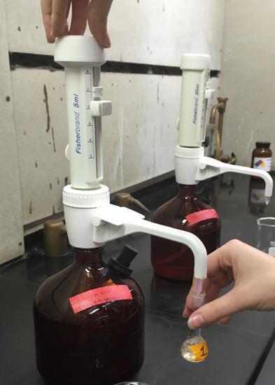 Using the dispenser, add the correct amount of \(\ce{KSCN}\) solution to each of the labeled flasks, according to the table below.
Step 4
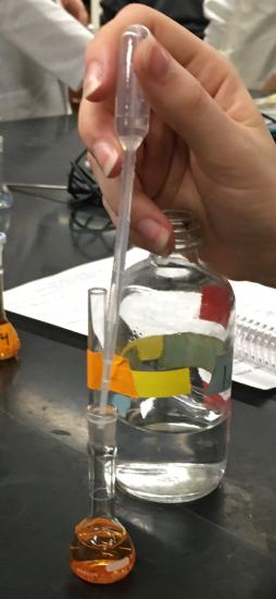 Fill the volumetric flasks to the line with \(\ce{HNO3}\). Mix each solution thoroughly by inverting the volumetric flasks several times.
Step 5
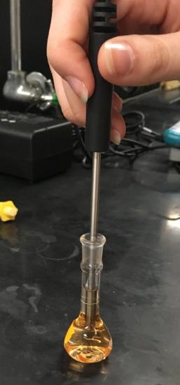 Take the temperature of one of the flasks using the Vernier Temperature Probe.
Table 2: Test Mixtures
| Mixture | \(\ce{Fe(NO3)3}\) Solution | \(\ce{KSCN}\) Solution |
|---|---|---|
| 1 | 5.00 mL | 2.00 mL |
| 2 | 5.00 mL | 3.00 mL |
| 3 | 5.00 mL | 4.00 mL |
| 4 | 5.00 mL | 5.00 mL |
Five solutions will be prepared from 2.00 x 10⁻³ M \(\ce{KSCN}\) and 2.00 x 10⁻³ M \(\ce{Fe(NO3)3}\) according to this table. If the mixtures are prepared properly, the solutions will gradually become lighter in color from the first to the fifth mixture. Use this table to perform dilution calculations to find the initial reactant concentrations to use in Figure 3.
Part B: Preparation of a Standard Solution of \(\ce{FeSCN^{2+}}\)
Prepare a standard solution with a known concentration of \(\ce{FeSCN^{2+}}\).
Step 1
Label a sixth clean and dry 10 mL volumetric flask as the standard.
Step 2
Add 1.00 mL of the \(\ce{KSCN}\) solution.
Step 3
Fill the remainder of the flask with 0.200 M \(\ce{FeNO3}\). (Note the different concentration of this solution.) Mix the solution thoroughly by inverting the flask. This solution should be darker than any of the other five solutions prepared previously.
Part C: Spectrophotometric Determination of \([\ce{FeSCN^{2+}}]\)
Step 1
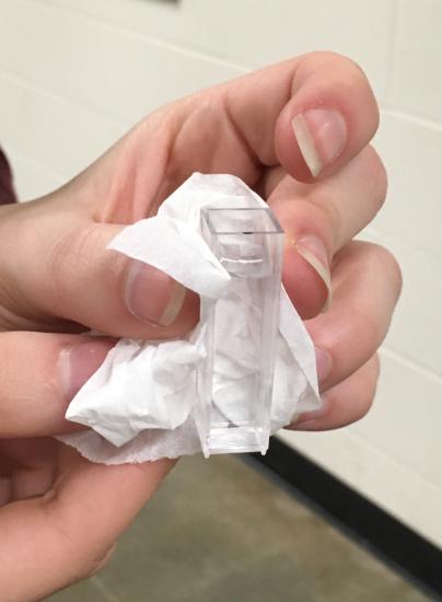 Fill a cuvet with distilled water and carefully wipe off the outside with a tissue.
Step 2
Insert the cuvet into the Vernier colorimeter. Be sure to make sure it is oriented correctly by aligning the mark on cuvet towards the arrow inside the colorimeter and close the lid.
Step 3
Select 470 nm as your wavelength by using the arrows on the colorimeter and press the calibrate button.
Step 4
 For each standard solution in Table 2, rinse your cuvet with a small amount of the standard solution to be measured, disposing the rinse solution in a waste beaker.
Step 5
Fill the cuvet with the standard, insert the cuvet as before and record the absorbance reading. Continue until all solutions have an absorbance reading.
Step 6
Dispose of all solutions in the waste container.
Calculations:
Part A: Initial concentrations of \(\ce{Fe^{3+}}\) and \(\ce{SCN^{-}}\) in Unknown Mixtures
Experimental Data
| Volumetric Flask | Reagent Volumes (mL) | Initial Concentrations (M) | |||
|---|---|---|---|---|---|
| -- | 2.00 x 10⁻³ M \(\ce{Fe(NO3)3}\) | 2.00 x 10⁻³ M \(\ce{KSCN}\) | Water | \(\ce{Fe^{3+}_{i}}\) | \(\ce{SCN^{-}_{i}}\) |
| 1 | 5.00 | 5.00 | 0.00 | ||
| 2 | 5.00 | 4.00 | 1.00 | ||
| 3 | 5.00 | 3.00 | 2.00 | ||
| 4 | 5.00 | 2.00 | 3.00 | ||
| 5 | 5.00 | 1.00 | 4.00 | ||
- Show a sample dilution calculation for (\(\ce{Fe^{3+}})_{i}\) and (\(\ce{SCN^{-}})_{i}\) initial in flask #1.
The Standard \(\ce{FeSCN^{2+}}\) Solution
Given 9.00 mL of 0.200 M \(\ce{Fe(NO3)3}\) and 1.00 mL of 0.00200 M \(\ce{KSCN}\), calculate the concentration of \([\ce{FeSCN^{2+}}]\).
- Equilibrium \([\ce{FeSCN^{2+}}]\) in Standard Solution: ______________ M
Note that since \([\ce{Fe^{3+}}]>>[\ce{SCN^{-}}]\) in the Standard Solution, the reaction is forced to completion, thus causing all the \(\ce{SCN^{-}}\) to convert to \(\ce{FeSCN^{2+}}\).
- Show the stoichiometry and dilution calculations used to obtain this value.
Test mixtures
| Mixture | Absorbance | \([\ce{FeSCN^{2+}_{eq}}]\) (M) |
|---|---|---|
| 1 | ||
| 2 | ||
| 3 | ||
| 4 | ||
| 5 |
- Show a sample calculation for \([\ce{FeSCN^{2+}}]\) in mixture 1.
Analysis
The reaction that is assumed to occur in this experiment is: \(\ce{Fe^{3+} (aq) + SCN^{-} (aq) <=> FeSCN^{2+} (aq)} \)
- Write the equilibrium constant expression for the reaction.
- Show a sample calculation for the value of \(K_{c}\) using the data for flask #1.
Using the same method you outlined above, complete the table for all the equilibrium concentrations and value of \(K_{c}\):
| Tube | Equilibrium Concentrations (M) | \(K_{c}\) | ||
|---|---|---|---|---|
| -- | \(\ce{Fe^{3+}_{eq}}\) | \(\ce{SCN^{-}_{eq}}\) | \(\ce{FeSCN^{2+}_{eq}}\) | -- |
| 1 | ||||
| 2 | ||||
| 3 | ||||
| 4 | ||||
- Average value of \(K_{c}\) ________________ (Use reasonable number of significant digits, based on the distribution of your \(K_{c}\) values.)