14.2: Magnetic Properties of Materials

 

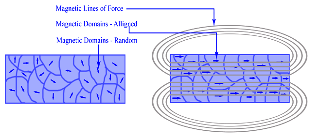
Ferromagnetism is the basic mechanism by which certain materials (such as iron) form permanent magnets. This means the compound shows permanent magnetic properties rather than exhibiting them only in the presence of a magnetic field (Figure \(\PageIndex{1}\)). In a ferromagnetic element, electrons of atoms are grouped into domains in which each domain has the same charge. In the presence of a magnetic field, these domains line up so that charges are parallel throughout the entire compound. Whether a compound can be ferromagnetic or not depends on its number of unpaired electrons and on its atomic size.

Figure \(\PageIndex{1}\): Ferromagnetism (a) nonmagnatized material and (2) Magnetized material with corresponding magnetic fields shown.

Ferromagnetism, the permanent magnetism associated with nickel, cobalt, and iron, is a common occurrence in everyday life. Examples of the knowledge and application of ferromagnetism include Aristotle's discussion in 625 BC, the use of the compass in 1187, and the modern-day refrigerator. Einstein declared that electricity and magnetism are inextricably linked in his theory of special relativity.

---

The magnetic moment of a system measures the strength and the direction of its magnetism. The term itself usually refers to the magnetic dipole moment. Anything that is magnetic, like a bar magnet or a loop of electric current, has a magnetic moment. A magnetic moment is a vector quantity, with a magnitude and a direction. An electron has an electron magnetic dipole moment, generated by the electron's intrinsic spin property, making it an electric charge in motion. There are many different magnetic forms: including paramagnetism, and diamagnetism, ferromagnetism, and anti-ferromagnetism. Only the first two are introduced below.

Paramagnetism

Paramagnetism refers to the magnetic state of an atom with one or more unpaired electrons. The unpaired electrons are attracted by a magnetic field due to the electrons' magnetic dipole moments. Hund's Rule states that electrons must occupy every orbital singly before any orbital is doubly occupied. This may leave the atom with many unpaired electrons. Because unpaired electrons can spin in either direction, they display magnetic moments in any direction. This capability allows paramagnetic atoms to be attracted to magnetic fields. Diatomic oxygen, \(O_2\) is a good example of paramagnetism (described via molecular orbital theory). The following video shows liquid oxygen attracted into a magnetic field created by a strong magnet:

A chemical demonstration of the paramagnetism of oxygen, as shown by the attraction of liquid oxygen to a magnet. Carleton University, Ottawa, Canada.

As shown in the video, molecular oxygen (\(O_2\) is paramagnetic and is attracted to the magnet. Incontrast, Molecular nitrogen, \(N_2\), however, has no unpaired electrons and it is diamagnetic (this concept is discussed below); it is therefore unaffected by the magnet.

There are some exceptions to the paramagnetism rule; these concern some transition metals, in which the unpaired electron is not in a d-orbital. Examples of these metals include \(Sc^{3+}\), \(Ti^{4+}\), \(Zn^{2+}\), and \(Cu^+\). These metals are the not defined as paramagnetic: they are considered diamagnetic because all d-electrons are paired. Paramagnetic compounds sometimes display bulk magnetic properties due to the clustering of the metal atoms. This phenomenon is known as ferromagnetism, but this property is not discussed here.

Diamagnetism

Diamagnetic substances are characterized by paired electrons—except in the previously-discussed case of transition metals, there are no unpaired electrons. According to the Pauli Exclusion Principle which states that no two identical electrons may take up the same quantum state at the same time, the electron spins are oriented in opposite directions. This causes the magnetic fields of the electrons to cancel out; thus there is no net magnetic moment, and the atom cannot be attracted into a magnetic field. In fact, diamagnetic substances are weakly repelled by a magnetic field. In fact, diamagnetic substances are weakly repelled by a magnetic field as demonstrated with the pyrolytic carbon sheet in Figure \(\PageIndex{6}\).

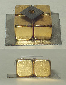
Figure \(\PageIndex{6}\): Levitating pyrolytic carbon: A small (~6 mm) piece of pyrolytic graphite levitating over a permanent neodymium magnet array (5 mm cubes on a piece of steel). Note that the poles of the magnets are aligned vertically and alternate (two with north facing up, and two with south facing up, diagonally). from Wikipedia.

How to Tell if a Substance is Paramagnetic or Diamagnetic

The magnetic form of a substance can be determined by examining its electron configuration: if it shows unpaired electrons, then the substance is paramagnetic; if all electrons are paired, the substance is diamagnetic. This process can be broken into four steps:

1. Find the electron configuration
2. Draw the valence orbitals
3. Look for unpaired electrons
4. Determine whether the substance is paramagnetic (one or more unpaired electrons) or diamagnetic (all electrons paired)

Example \(\PageIndex{4}\): Chlorine atoms

Are chlorine atoms paramagnetic or diamagnetic?

Solution

Step 1: Find the electron configuration

For Cl atoms, the electron configuration is 3s²3p⁵

Step 2: Draw the valence orbitals

Ignore the core electrons and focus on the valence electrons only.

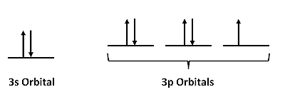
Step 3: Look for unpaired electrons

There is one unpaired electron.

Step 4: Determine whether the substance is paramagnetic or diamagnetic

Since there is an unpaired electron, Cl atoms are paramagnetic (but is quite weak).

Example 2: Zinc Atoms

Step 1: Find the electron configuration

For Zn atoms, the electron configuration is 4s²3d¹⁰

Step 2: Draw the valence orbitals

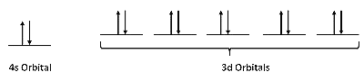
Step 3: Look for unpaired electrons

There are no unpaired electrons.

Step 4: Determine whether the substance is paramagnetic or diamagnetic

Because there are no unpaired electrons, Zn atoms are diamagnetic.

---

The magnetism of metals and other materials are determined by the orbital and spin motions of the unpaired electrons and the way in which unpaired electrons align with each other. All magnetic substances are paramagnetic at sufficiently high temperature, where the thermal energy (kT) exceeds the interaction energy between spins on neighboring atoms. Below a certain critical temperature, spins can adopt different kinds of ordered arrangements.

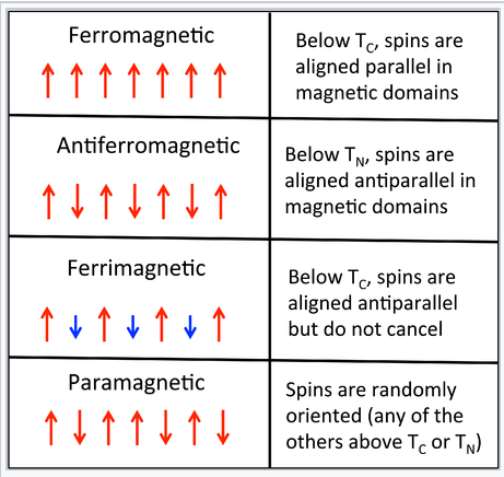
A pictorial description of the ordering of spins in ferromagnetism, antiferromagnetism, ferrimagnetism, and paramagnetism

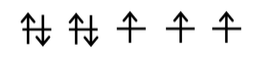
Let's begin by considering an individual atom in the bcc structure of iron metal. Fe is in group VIIIb of the periodic table, so it has eight valence electrons. The atom is promoted to the 4s¹3d⁷ state in order to make bonds. A localized picture of the d-electrons for an individual iron atom might look like this:

Since each unpaired electron has a spin moment of 1/2, the total spin angular momentum, S, for this atom is:

\(S = 3\frac{1}{2} = \frac{3}{2}\) (in units of h/2π)

We can think of each Fe atom in the solid as a little bar magnet with a spin-only moment S of 3/2. The spin moments of neigboring atoms can align in parallel (↑ ↑), antiparallel (↑ ↓), or random fashion. In bcc Fe, the tendency is to align parallel because of the positive sign of the exchange interaction. This results in ferromagnetic ordering, in which all the spins within a magnetic domain (typically hundreds of unit cells in width) have the same orientation, as shown in the figure at the right. Conversely, a negative exchange interaction between neighboring atoms in bcc Cr results in antiferromagnetic ordering. A third arrangement, ferrimagnetic ordering, results from an antiparallel alignment of spins on neighboring atoms when the magnetic moments of the neighbors are unequal. In this case, the spin moments do not cancel and there is a net magnetization. The ordering mechanism is like that of an antiferromagnetic solid, but the magnetic properties resemble those of a ferromagnet. Ferrimagnetic ordering is most common in metal oxides, as we will learn in Chapter 7.

Magnetization and susceptibility

The magnetic susceptibility, χ, of a solid depends on the ordering of spins. Paramagnetic, ferromagnetic, antiferromagnetic, and ferrimagnetic solids all have χ > 0, but the magnitude of their susceptibility varies with the kind of ordering and with temperature. We will see these kinds of magnetic ordering primarily among the 3d and 4f elements and their alloys and compounds. For example, Fe, Co, Ni, Nd₂Fe₁₄B, SmCo₅, and YCo₅ are all ferromagnets, Cr and MnO are antiferromagnets, and Fe₃O₄ and CoFe₂O₄ are ferrimagnets. Diamagnetic compounds have a weak negative susceptibility (χ < 0).

Definitions

• H = applied magnetic field (units: Henry (H))
• B = induced magnetic field in a material (units: Tesla (T))
• M = magnetization, which represents the magnetic moments within a material in the presence of an external field H.

Magnetic susceptibility χ = M/H

Usually, χ is given in molar units in the cgs system:

χ_M = molar susceptibility (units: cm³/mol)

Typical values of χ_M:

Compound	Type of Magnetism	χ at 300K (cm^3/mol)
SiO2	Diamagnetic	- 3 x 10^-4
Pt metal	Pauli paramagnetic	+ 2 x 10^-4
Gd2(SO4)3^.8H2O	Paramagnetic	+ 5 x 10^-2
Ni-Fe alloy	Ferromagnetic	+ 10^4 - 10^6

To correlate χ with the number of unpaired electrons in a compound, we first correct for the small diamagnetic contribution of the core electrons:

\[\chi^{corr} = \chi^{obs}- \chi^{diamagnetic\: cores}\]

Susceptibility of paramagnets

For a paramagnetic substance,

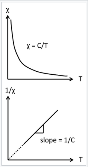
\[\chi^{corr}_{M} = \frac{C}{T}\]

The inverse relationship between the magnetic susceptibility and T, the absolute temperature, is called Curie's Law, and the proportionality constant C is the Curie constant:

\[C= \frac{N_{A}}{3k_{B}}\mu^{2}_{eff}\]

Note that C is not a "constant" in the usual sense, because it depends on µ_eff, the effective magnetic moment of the molecule or ion, which in turn depends on its number of unpaired electrons:

\[\mu_{eff} = \sqrt{n(n+2)}\mu_{B}\]

Curie law behavior of a paramagnet. A plot of 1/χ vs. absolute temperature is a straight line, with a slope of 1/C and an intercept of zero.

Here µ_B is the Bohr magneton, a physical constant defined as µ_B = eh/4πm_e = 9.274 x 10^-21 erg/gauss (in cgs units).

In cgs units, we can combine physical constants,

\[\frac{N_{A}}{3k_{B}} \mu^{2}_{B} = .125\]

Combining these equations, we obtain

\[\chi^{corr}_{M} = \frac{.125}{T}(\frac{\mu_{eff}}{\mu_{B}})^{2}\]

These equations relate the molar susceptibility, a bulk quantity that can be measured with a magnetometer, to µ_eff, a quantity that can be calculated from the number of unpaired electrons, n. Two important points to note about this formula are:

• The magnetic susceptibility is inversely proportional to the absolute temperature, with a proportionality constant C (Curie's Law)
• So far we are talking only about paramagnetic substances, where there is no interaction between neighboring atoms.

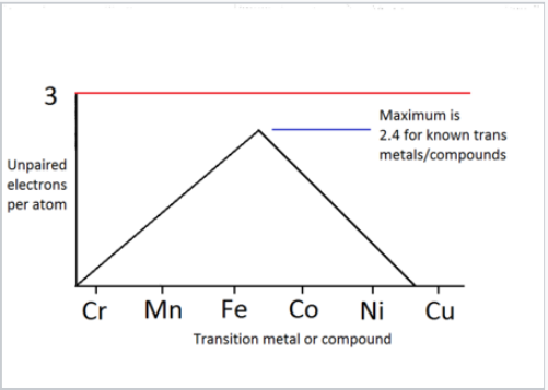
Number of unpaired electrons per atom, determined from Curie constants of transition metals and their 1:1 alloys.

Returning to the isolated Fe atom with its three unpaired electrons, we can measure the Curie constant for iron metal (above the temperature of its transition to a paramagnetic solid) and compare it to the calculation of µ_eff. Since n = 3, we calculate:

\[\mu_{eff}= \sqrt{(3)(5)} \mu_{B} = 3.87\mu_{B}\]

The plot at the right shows the number of unpaired electrons per atom, calculated from measured Curie constants, for the magnetic elements and 1:1 alloys in the 3d series. The plot peaks at a value of 2.4 spins per atom, slightly lower than we calculated for an isolated iron atom. This reflects that fact that there is some pairing of d-electrons, i.e., that they do contribute somewhat to bonding in this part of the periodic table.

Susceptibility of ferro-, ferri-, and antiferromagnets

Below a certain critical temperature, the spins of a solid paramagnetic substance order and the susceptibility deviates from simple Curie-law behavior. Because the ordering depends on the short-range exchange interaction, this critical temperature varies widely. Metals and alloys in the 3d series tend to have high critical temperatures because the atoms are directly bonded to each other and the interaction is strong. For example, Fe and Co have critical temperatures (also called the Curie temperature, T_c, for ferromagnetic substances) of 1043 and 1400 K, respectively. The Curie temperature is determined by the strength of the magnetic exchange interaction and by the number of unpaired electrons per atom. The number of unpaired electrons peaks between Fe and Co as the d-band is filled, and the exchange interaction is stronger for Co than for Fe. In contrast to ferromagnetic metals and alloys, paramagnetic salts of transition metal ions typically have critical temperatures below 1K because the magnetic ions are not directly bonded to each other and thus their spins are very weakly coupled in the solid state. For example, in gadolinium sulfate, the paramagnetic Gd³⁺ ions are isolated from each other by SO₄^2- ions.

Magnetic susceptibility vs temperature (Kelvin) for ferrimagnetic, ferromagnetic, and antiferromagnetic materials

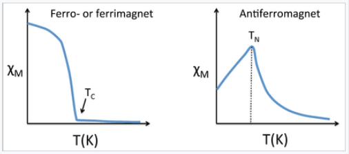
Above the critical temperature T_C, ferromagnetic compounds become paramagnetic and obey the Curie-Weiss law:

\[\chi= \frac{C}{T-T_{c}}\]

This is similar to the Curie law, except that the plot of 1/χ vs. T is shifted to a positive intercept T_C on the temperature axis. This reflects the fact that ferromagnetic materials (in their paramagnetic state) have a greater tendency for their spins to align in a magnetic field than an ordinary paramagnet in which the spins do not interact with each other. Ferrimagnets follow the same kind of ordering behavior. Typical plots of χ vs. T and 1/χ vs. T for ferro-/ferrimagnets are shown above and below.

Plots of 1/χ vs. T for ferromagnets, ferrimagnets, and antiferromagnets.

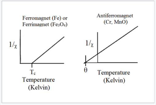
Antiferromagnetic solids are also paramagnetic above a critical temperature, which is called the Néel temperature, T_N. For antiferromagnets, χ reaches a maximum at T_N and is smaller at higher temperature (where the paramagnetic spins are further disordered by thermal energy) and at lower temperature (where the spins pair up). Typically, antiferromagnets retain some positive susceptibility even at very low temperature because of canting of their paired spins. However the maximum value of χ is much lower for an antiferromagnet than it is for a ferro- or ferrimagnet. The Curie-Weiss law is also modified for an antiferromagnet, reflecting the tendency of spins (in the paramagnetic state above T_N) to resist parallel ordering. A plot of 1/χ vs. T intercepts the temperature axis at a negative temperature, -θ, and the Curie-Weiss law becomes:

\[\chi= \frac{C}{T + \theta}\]

Ordering of spins below T_C

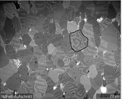
Below T_C, the spins align spontaneously in ferro- and ferrimagnets. Complex magnetization behavior is observed that depends on the history of the sample. For example, if a ferromagnetic material is cooled in the absence of an applied magnetic field, it forms a mosaic structure of magnetic domains that each have internally aligned spins. However, neighboring domains tend to align the opposite way in order to minimize the total energy of the system. This is illustrated in the figure at the left for a Nd-Fe-B magnet. The sample consists of 5-10 µm wide crystal grains that can be easily distinguished by the sharp boundaries in the image. Within each grain are a series of lighter and darker stripes (imaged by using the optical Kerr effect) that are ferromagnetic domains with opposite orientations. Averaged over the whole sample, these domains have random orientation so the net magnetization is zero.

Microcrystalline grains within a piece of Nd2Fe14B (the alloy used in neodymium magnets) with magnetic domains made visible with a Kerr microscope. The domains are the light and dark stripes visible within each grain.

When a sample like this one is magnetized (i.e., exposed to a strong magnetic field), the domain walls move and the favorably aligned domains grow at the expense of those with the opposite orientation. This transformation can be seen in real time in the Kerr microscope. The domain walls are typically hundreds of atoms wide, so movement of a domain wall involves a cooperative tilting of spin orientation (analogous to "the wave" in a sports stadium) and is a relatively low energy process.

The movement of domain walls in a grain of silicon steel is driven in this movie by increasing the external magnetic field in the "downward" direction, and is imaged using a Kerr microscope. White areas are domains with their magnetization directed up, dark areas - which eventually comprise the entire grain - are domains with their magnetization directed down.

The process of magnetization moves the solid away from its lowest energy state (random domain orientation), so magnetization involves input of energy. When the external magnetic field is removed, the domain walls relax somewhat, but the solid (especially in the case of a "hard" magnet) can retain much of its magnetization. If you have ever magnetized a nail or a paper clip by using a permanent magnet, what you were doing was moving the walls of the magnetic domains inside the ferromagnet. The object thereafter retains the "memory" of its magnetization. However, annealing a permanent magnet destroys the magnetization by returning the system to its lowest energy state in which all the magnetic domains cancel each other.

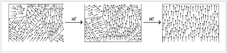
Rotation of orientation and increase in size of magnetic domains in response to an externally applied magnetic field.

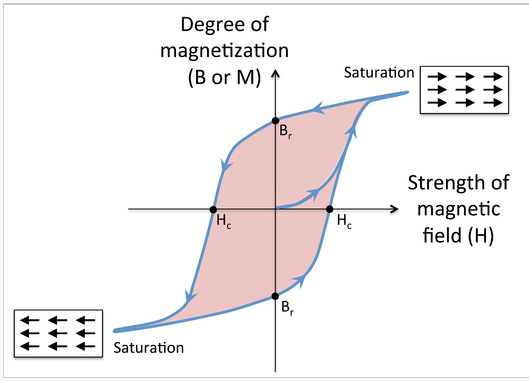
Magnetic hysteresis. Cycling a ferro- or ferrimagnetic material in a magnetic field results in hysteresis in the magnetization of the material, as shown in the figure at the left. At the beginning, the magnetization is zero, but it begins to rise rapidly as the magnetic field is applied. At high field, the magnetic domains are aligned and the magnetization is said to be saturated. When the field is removed, a certain remanent magnetization (indicated as the point B_r on the graph) is retained, i.e., the material is magnetized. Applying a field in the opposite direction begins to orient the magnetic domains in the other direction, and at a field H_c (the coercive field), the magnetization of the sample is reduced to zero. Eventually the material reaches saturation in the opposite direction, and when the field is removed again, it has remanent magnetization Br, but in the opposite direction. As the field continues to reverse, the magnet follows the hysteresis loop as indicated by the arrows. The area of colored region inside the loop is proportional to the magnetic work done in each cycle. When the field cycles rapidly (for example, in the core of a transformer, or in read-write cycles of a magnetic disk) this work is turned into heat.

Magnetization of a ferro- or ferrimagnet vs. applied magnetic field H. Starting at the origin, the upward curve is the initial magnetization curve. The downward curve after saturation, along with the lower return curve, form the main loop. The intercepts Hc and Br are the coercivity and remanent magnetization.

Contributors and Attributions

• Neele Holzenkaempfer, Jesse Gipe

• Chris P Schaller, Ph.D., (College of Saint Benedict / Saint John's University)

• Paul Flowers (University of North Carolina - Pembroke), Klaus Theopold (University of Delaware) and Richard Langley (Stephen F. Austin State University) with contributing authors. Textbook content produced by OpenStax College is licensed under a Creative Commons Attribution License 4.0 license. Download for free at http://cnx.org/contents/85abf193-2bd...a7ac8df6@9.110).

• Jim Clark (Chemguide.co.uk)

• Dr. Richard Spinney (The Ohio State University)