4.2.2: Orbital Mixing

CHEM 431: Inorganic Chemistry
Fall 2020: Dr. Kathryn Haas

 Home    ●   Readings   ●  Course Info & Tools 

---

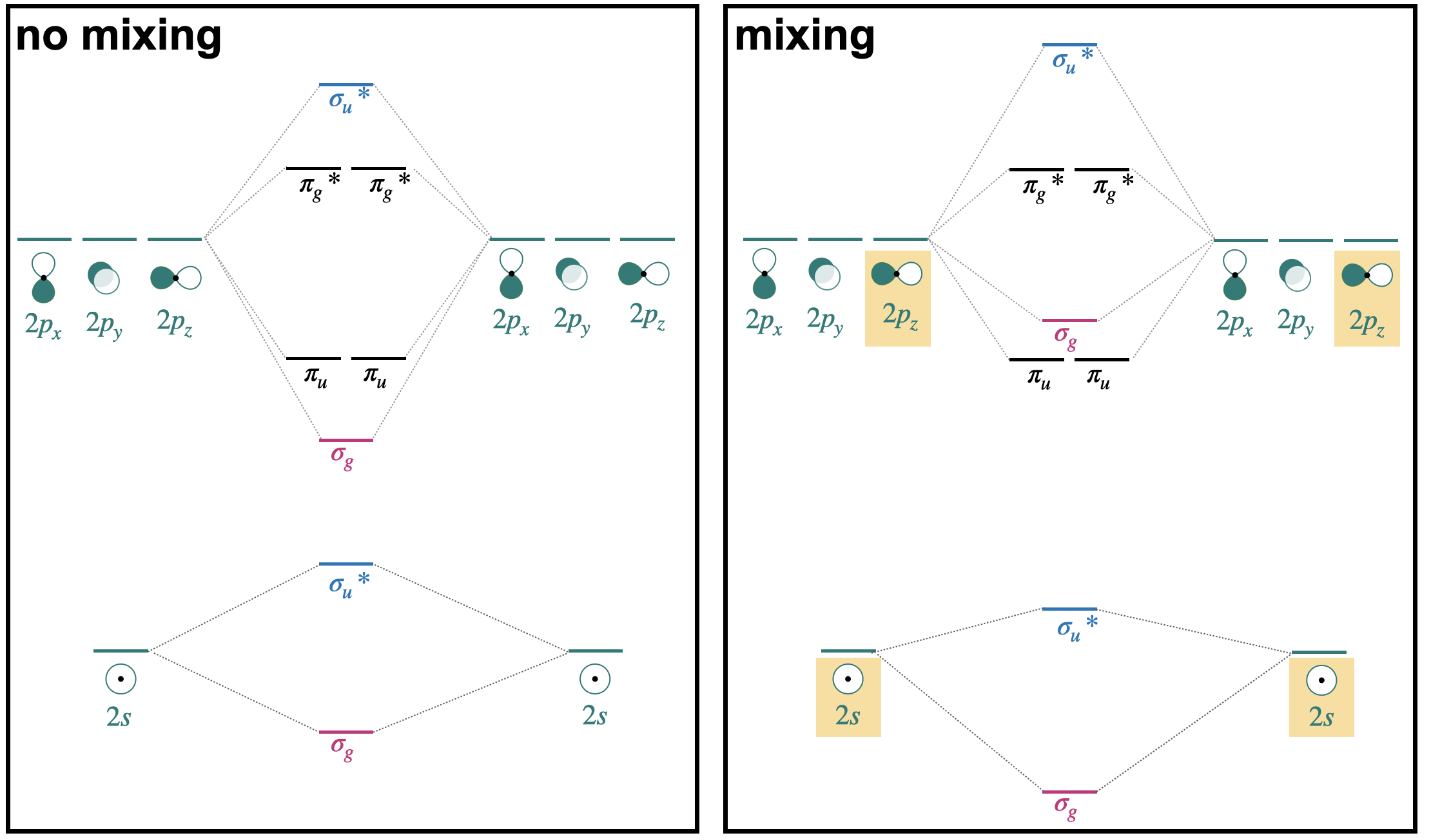
In the previous section, we introduced a simplified molecular orbital (MO) diagram, assuming that interactions were limited to degenerate orbitals of compatible symmetry. A version of that diagram for second-row homonuclear diatomics is shown on the right side of Figure \(\PageIndex{1}\) (only valence orbitals shown).

In reality, orbitals of compatible symmetry can combine, or mix, even when they have different energies. When sets of orbitals mix, it has the effect of decreasing the energy of the lower-energy set and increasing the energy of the higher-energy set. There are two ways to explain mixing, described in the points below. The diagram on the right of side of Figure \(\PageIndex{1}\) shows how energy levels are affected by orbital mixing. 

• Starting from the simplified MO diagram and mixing molecular orbitals of like symmetry: If we start with the simplified diagram shown on the right, we can pick out the orbitals with like symmetry and consider what will happen if these molecular orbitals mix. For example, starting from the MO diagram on the right side of Figure \(\PageIndex{1}\), we see that there are two \(\sigma_g\) orbitals that have identical symmetry (hence they have identical symmetry labels). Upon mixing, the lower-energy \(\sigma_g(2s)\) will decrease in energy while the higher-energy \(\sigma_g(2p)\) will increase in energy. Likewise, there are two \(\sigma_u*\) orbitals that will mix, decreasing the energy of \(\sigma_u*(2s)\) while increasing the energy of \(\sigma_u*(2p)\).
• Starting from and mixing atomic orbitals of compatible symmetry: Starting from the atomic orbitals, we can select the orbitals that have compatible symmetry to make productive interactions, and combine them as a set to make molecular orbitals. From the two sets of atomic orbitals on the right panel in Figure (\PageIndex{1}\), there are two sets of four orbitals with compatable symmetry; one is the set of two \(2s\) and two \(2p_z\) orbitals. These four orbitals can combine to form molecular orbitals with \(\sigma\) symmetry. They combine to form one lowest-energy bonding \(\sigma_g\), a highest-energy \(\sigma_u*\), and two orbitals with intermediate energy (\(\sigma_g\), and \(\sigma_u*\)). This treatment can be xpressed as the linear combination of four atomic orbitals:
  \[\Psi=c_{1} \psi\left(2 s_{a}\right) \pm c_{2} \psi\left(2 s_{b}\right) \pm c_{3} \psi\left(2 p_{a}\right) \pm c_{4} \psi\left(2 p_{b}\right)\]
  where the coefficients \(c_1=c_2\) and \(c_3=c_4\) for homonuclear diatomic molecues.

 

Figure \(\PageIndex{1}\): Mixing of orbitals with like symmetry affects the energies of molecular orbitals. 

In the case of homonuclear diatomic molecules of the second row, orbital mixing has important consequences for the energetic order of the \(\sigma_g(2p\) and \(\pi_u(2p)\) orbitals. This will be discussed in the next section.

Curated or created by Kathryn Haas