8.3: The Effects of Instumental Noise on Spectrophotometric Analyses

The Relationship Between the Uncertainty in c and the Uncertainty in T

The accuracy and precision of quantitative spectrochemical analysis with Beer's Law are often limited by the uncertainties or electrical noise associated with the instrument and its components (source, detector, amplifiers, etc.).

Starting with Beer's Law we can write the following expressions for c

\(c=-\frac{1}{\varepsilon b} \log T=-\frac{0.434}{\varepsilon b} \ln T\)

taking the partial derivative of c with respect to T and holding b and [\epsilon} constant yeilds

\(\frac{\partial c}{\partial T}=-\frac{0.434}{\varepsilon b T}\)

converting from standard deviations to variances yeilds

\(\sigma_{c}^{2}=\left(\frac{\partial c}{\partial T}\right)^{2} \sigma_{T}^{2}=\left(\frac{-0.434}{\delta D T}\right)^{2} \sigma_{T}^{2}\)

and dividing the square of the first expression for c results in the equation below involving the variance in c and the variance in T

\(\left(\frac{\sigma_{c}}{c}\right)^{2}=\left(\frac{\sigma_{T}}{T \ln T}\right)^{2}\)

Taking the square root of both sides yields the equation below for the relative uncertainty in c 

\(\frac{\sigma_{c}}{c}=\frac{\sigma_{T}}{T \ln T}=\frac{0.434 \sigma_{T}}{T \log T}\)

For a limited number of measurements one replaces the standard deviations of the population, \({\sigma}\), with the standard deviations of the sample, s, and obtain

\(\frac{s_{c}}{c}=\frac{0.434 s_{r}}{T \log T}\)

This last equation relates the relative standard deviation (relative uncertainty) of c to the absolute standard deviation of T, s_T.  Experimentally s_T can be evaluated by repeatedly measuring T for the same sample.   The last equation also shows that the relative uncertainty in c varies nonlinearly with the magnitude of T.  

It should be noted that the last equation for the relative uncertainty in c understates the complexity of this problem as the uncertainty in T, s_T is is many circumstances dependent on the magnitude of T.

Sources of Instrumental Noise

In a detailed theoretical and experimental study Rothman, Crouch, and Ingle (Anal. Chem 47, 1226 (1975)) described several sources of instrumental uncertainties and showed their net effect on the precision of transmittance measurements.   As shown in the table below, these uncertainties fall into three categories depending on how affected they are by the magnitude of T

Category	Characterized by sT  =	Typical sources for UV/Vis experiments	Likely to be important in
1	k1	limited readout resolution Dark current and amplifier noise	low cost instruments with meters or few digits in display regions where source intensity and detector sensitivity is low
2	\(k_{2} \sqrt{T^{2}+T}\)	Photon detector shot noise	High quality instruments with photomultiplier tubes
3	k3T	cell positioning uncertainty Source flick noise	High quality instruments low cost instruments

Category 1: s_T = k₁

Low cost instruments which in the past might have had analog meter movements or possibly available today 4 digits (reporting %T with values ranging from 0.0 to 100.0) are instruments where the readout error is on the order of 0.2 %T.  The magnitude of this error is larger that should be expected from detector and amplifier noise except under the condition where the source intensity or detector sensitivity is low (little light being measured by the detector). 

Substitution of s_T = k1 yields 

\(\frac{s_{c}}{c}=\frac{0.434 k_{1}}{T \log T}\)

and evaluating this equation over the range of T = 0.95 to 0.001 (corresponding A values 0.022 to 3.00) and using a reasonable value for k₁ such as 0.003 or 0.3 %T  is shown as the red curve in Figure 8.3.1.  Looking carefully at the red curve the relative uncertainty is at best on the order of 1.0% and gets considerably larger as the T increases (A decreases) or T decreases (A increases).  These ends of the "U" shaped curve correspond to situations where not much light is absorbed and P is very close to P₀ or when most of the light is absorbed and P is very small). 

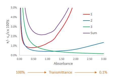
Figure \(\PageIndex{1}\): The relative uncertainty in c for different values of T or A in accord with the three Categories of instrument noise affect measurements of T. 

Category 2: \(s_{T}=k_{2} \sqrt{T^{2}+T}\)

The type of uncertainty described by Category 2 is associated with the highest quality instruments containing the most sensitive light detector s.  Photon shot noise is observed when ever an electron moves across a junction such as the movement of an electron from the photocathode to the first dynode in a photomultiplier tube.  In these cases the current results from a series of discrete events the number of which per unit time is distributed in a random way about a mean value.  The magnitude of the current fluctuations is proportional to the square root of the current.  Therefore for Category 2 \(s_{T}=k_{2} \sqrt{T^{2}+T}\)  and 

\(\frac{s_{c}}{c}=\frac{0.434 \times k_{2}}{\log T} \sqrt{\frac{1}{T}+1}\)

An evaluation of s_c/c for Category 2, as done for Category 1, is shown in the blue curve in figure 8.3.1 where k₂ = 0.003.  The contribution of the uncertainty associated with Category 2 is largest when the T is large and the A is low.  Under these conditions the photocurrent in the detector is large as a great deal of light is striking the detector. 

Category 3: s_T = k₃

The most common phenomena associated with the Category 3 uncertainty in the measurement of T is flicker noise.  Flicker noise, or 1/f noise, is often associated with the slow drift in source intensity, P₀.  Instrument makers address flicker noise by either regulating the power to the optical source, designing a double beam spectrophotometer where the light path of a single source alternates between passing through the sample or a reference, or both. 

Another  widely encountered noise associated with Category 3 is the failure to position the sample and or reference cells is exactly the same place each time.  Even the highest quality cuvettes will have some scattering imperfections in the cuvette material and other scattering sources can be dust particles on the cuvette surface and finger smudges.  One method to reduce the problems associated with cuvette positioning is to leave the cuvettes in place and carefully change the samples with rinsing using disposable pipets.  In their paper mentioned earlier, Rothman, Crouch and Ingle argue that this is the largest source of error for experiments with high quality spectrophotometer.

The effect of the Category 3 uncertainty where s_T = k₃T is revealed by green curve in Figure 8.2.1. 

\(\frac{s_{c}}{c}=\frac{0.434 \times k_{3}}{\log T}\)

In this case k₃ = 0.0013 and like Category 2 the contribution of Category 3 uncertainty to the relative uncertainty in c is largest when T is large and A is small.

The purple curve in Figure 8.2.1 is the sum of the contribution of Categories 1, 2 and 3.   The shape of the curve is very much like the Category 1 curve shown in red.  The relative uncertainty is largest when T is large (small A) or when T is small (large A).  The curve has a minimum near T = 0.2 (or % T = 20%) or A = 0.7 and most analytical chemists will try to get there calibration curve standards to have A values between 0.1 and 1.

The Effect of Slit Width on Absorbance Measurements

As presented in Section 7.3, the bandwidth of a wavelength selector is the product of the reciprocal linear dispersion and the slit width, D^-1 W.  It can be readily observed that increasing the bandwidth of the light passing through the wavelength selector result in a loss of detail, fine structure, in the absorbance spectrum provided the sample has revealable fine structure.  Most molecules and complex ions in solution do not have observable fine structure but gas phase analytes, some rigid aromatic molecules and species containing lanthanides or actinides do.

For systems with observable fine structure the bandwdith set through the slit width, W, must be matched to the system.  However, a decrease in slit width is accompanied by a second order decrease in the radiant power emanating from the wavelength selector and available to interrogate the sample.  At very narrow slit widths spectral detail can be lost due to a decrease in signal to noise, especially at wavelengths when the source intensity or the detector response in low. 

In general it is a good practice to decrease the slit width and decrease the bandwidth no more that necessary.  In most benchtop instruments the slit width is an adjustable parameter and the slits can be sequentially narrowed until the absorbance peaks heights become constant.