8.2: Beer's Law

Absorbance and Concentration: Beer's Law

When monochromatic electromagnetic radiation passes through an infinitesimally thin layer of sample of thickness dx, it experiences a decrease in its power of dP (Figure  \(\PageIndex{8}\)).

Figure \(\PageIndex{1}\). Factors used to derive the Beer’s law.

This fractional decrease in power is proportional to the sample’s thickness and to the analyte’s concentration, C; thus

\[-\frac{d P}{P}=\alpha C d x \label{8.1}\]

where P is the power incident on the thin layer of sample and \(\alpha\) is a proportionality constant. Integrating the left side of equation \ref{8.1} over the sample’s full thickness

\(-\int_{P=P_{0}}^{P=P_{\mathrm{T}}} \frac{d P}{P}=\alpha C \int_{x=0}^{x=b} d x \)                Equation 8.2.2a

gives 

\( \ln \left(\frac{P_{0}}{P_{\mathrm{T}}}\right)=\alpha b C \)               Equation 8.2.2b

converting from ln to log, and substituting into equation 8.2.2b, gives

\[A=a b C \label{8.3}\]

where a is the analyte’s absorptivity with units of cm^–1 conc^–1. If we express the concentration using molarity, then we replace a with the molar absorptivity, \(\varepsilon\), which has units of cm^–1 M^–1.

\[A=\varepsilon b C \label{8.4}\]

The absorptivity and the molar absorptivity are proportional to the probability that the analyte absorbs a photon of a given energy. As a result, values for both a and \(\varepsilon\) depend on the wavelength of the absorbed photon.

Example \(\PageIndex{2}\)

A \(5.00 \times 10^{-4}\) M solution of analyte is placed in a sample cell that has a pathlength of 1.00 cm. At a wavelength of 490 nm, the solution’s absorbance is 0.338. What is the analyte’s molar absorptivity at this wavelength?

Solution

Solving equation \ref{8.4} for \(\epsilon\) and making appropriate substitutions gives

\[\varepsilon=\frac{A}{b C}=\frac{0.338}{(1.00 \ \mathrm{cm})\left(5.00 \times 10^{-4} \ \mathrm{M}\right)}=676 \ \mathrm{cm}^{-1} \ \mathrm{M}^{-1} \nonumber\]

Exercise \(\PageIndex{2}\)

A solution of the analyte from Example \(\PageIndex{2}\) has an absorbance of 0.228 in a 1.00-cm sample cell. What is the analyte’s concentration?

Answer

Making appropriate substitutions into Beer’s law

\[A=0.228=\varepsilon b C=\left(676 \ \mathrm{M}^{-1} \ \mathrm{cm}^{-1}\right)(1 \ \mathrm{cm}) C \nonumber\]

and solving for C gives a concentration of \(3.37 \times 10^{-4}\) M.

Equation 8.2.3 and equation 8.2.4, which establish the linear relationship between absorbance and concentration, are known as Beer’s law. Calibration curves based on Beer’s law are common in quantitative analyses.

As is often the case, the formulation of a law is more complicated than its name suggests. This is the case, for example, with Beer’s law, which also is known as the Beer-Lambert law or the Beer-Lambert-Bouguer law. Pierre Bouguer, in 1729, and Johann Lambert, in 1760, noted that the transmittance of light decreases exponentially with an increase in the sample’s thickness.

\[T \propto e^{-b} \nonumber\]

Later, in 1852, August Beer noted that the transmittance of light decreases exponentially as the concentration of the absorbing species increases.

\[T \propto e^{-C} \nonumber\]

Together, and when written in terms of absorbance instead of transmittance, these two relationships make up what we know as Beer’s law.

Beer's Law and Multicomponent Samples

We can extend Beer’s law to a sample that contains several absorbing components. If there are no interactions between the components, then the individual absorbances, A_i, are additive. For a two-component mixture of analyte’s X and Y, the total absorbance, A_tot, is

\[A_{tot}=A_{X}+A_{Y}=\varepsilon_{X} b C_{X}+\varepsilon_{Y} b C_{Y} \nonumber\]

Generalizing, the absorbance for a mixture of n components, A_mix, is

\[A_{m i x}=\sum_{i=1}^{n} A_{i}=\sum_{i=1}^{n} \varepsilon_{i} b C_{i} \label{10.6}\]

Limitations to Beer's Law

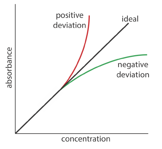
Beer’s law suggests that a plot of absorbance vs. concentration—we will call this a Beer’s law plot—is a straight line with a y-intercept of zero and a slope of ab or \(\varepsilon b\). In some cases a Beer’s law plot deviates from this ideal behavior (see Figure \(\PageIndex{9}\)), and such deviations from linearity are divided into three categories: fundamental, chemical, and instrumental.

Figure \(\PageIndex{2}\). Plots of absorbance vs. concentration showing positive and negative deviations from the ideal Beer’s law relationship, which is a straight line.

Fundamental Limitations to Beer's Law

Beer’s law is a limiting law that is valid only for low concentrations of analyte. There are two contributions to this fundamental limitation to Beer’s law. At higher concentrations the individual particles of analyte no longer are independent of each other. The resulting interaction between particles of analyte may change the analyte’s absorptivity. A second contribution is that an analyte’s absorptivity depends on the solution’s refractive index. Because a solution’s refractive index varies with the analyte’s concentration, values of a and \(\varepsilon\) may change. For sufficiently low concentrations of analyte, the refractive index essentially is constant and a Beer’s law plot is linear.

Chemical Limitations to Beer's Law

A chemical deviation from Beer’s law may occur if the analyte is involved in an equilibrium reaction. Consider, for example, the weak acid, HA. To construct a Beer’s law plot we prepare a series of standard solutions—each of which contains a known total concentration of HA—and then measure each solution’s absorbance at the same wavelength. Because HA is a weak acid, it is in equilibrium with its conjugate weak base, A^–.

In the equations that follow, the conjugate weak base A^– is written as A as it is easy to mistake the symbol for anionic charge as a minus sign.

\[\mathrm{HA}(a q)+\mathrm{H}_{2} \mathrm{O}(l)\rightleftharpoons\mathrm{H}_{3} \mathrm{O}^{+}(a q)+\mathrm{A}^{-}(a q) \nonumber\]

If both HA and A^– absorb at the selected wavelength, then Beer’s law is 

\[A=\varepsilon_{\mathrm{HA}} b C_{\mathrm{HA}}+\varepsilon_{\mathrm{A}} b C_{\mathrm{A}} \label{10.7}\]

Because the weak acid’s total concentration, C_total, is

\[C_{\mathrm{total}}=C_{\mathrm{HA}}+C_{\mathrm{A}} \nonumber\]

we can write the concentrations of HA and A^– as

\[C_{\mathrm{HA}}=\alpha_{\mathrm{HA}} C_{\mathrm{total}} \label{10.8}\]

\[C_{\text{A}} = (1 - \alpha_\text{HA})C_\text{total} \label{10.9}\]

where \(\alpha_\text{HA}\) is the fraction of weak acid present as HA. Substituting equation \ref{10.8} and equation \ref{10.9} into equation \ref{10.7} and rearranging, gives

\[A=\left(\varepsilon_{\mathrm{HA}} \alpha_{\mathrm{HA}}+\varepsilon_{\mathrm{A}}-\varepsilon_{\mathrm{A}} \alpha_{\mathrm{A}}\right) b C_{\mathrm{total}} \label{10.10}\]

To obtain a linear Beer’s law plot, we must satisfy one of two conditions. If \(\varepsilon_\text{HA}\) and \(\varepsilon_{\text{A}}\) have the same value at the selected wavelength, then equation \ref{10.10} simplifies to

\[A = \varepsilon_{\text{A}}bC_\text{total} = \varepsilon_\text{HA}bC_\text{total} \nonumber\]

Alternatively, if \(\alpha_\text{HA}\) has the same value for all standard solutions, then each term within the parentheses of equation \ref{10.10} is constant—which we replace with k—and a linear calibration curve is obtained at any wavelength.

\[A=k b C_{\mathrm{total}} \nonumber\]

Because HA is a weak acid, the value of \(\alpha_\text{HA}\) varies with pH. To hold \(\alpha_\text{HA}\) constant we buffer each standard solution to the same pH. Depending on the relative values of \(\alpha_\text{HA}\) and \(\alpha_{\text{A}}\), the calibration curve has a positive or a negative deviation from Beer’s law if we do not buffer the standards to the same pH.

Instrumental Limitations to Beer's Law

There are two principal instrumental limitations to Beer’s law. The first limitation is that Beer’s law assumes that radiation reaching the sample is of a single wavelength—that is, it assumes a purely monochromatic source of radiation. As shown in Figure 10.1.10, even the best wavelength selector passes radiation with a small, but finite effective bandwidth. Polychromatic radiation always gives a negative deviation from Beer’s law, but the effect is smaller if the value of \(\varepsilon\) essentially is constant over the wavelength range passed by the wavelength selector. For this reason, as shown in Figure \(\PageIndex{10}\), it is better to make absorbance measurements at the top of a broad absorption peak. In addition, the deviation from Beer’s law is less serious if the source’s effective bandwidth is less than one-tenth of the absorbing species’ natural bandwidth [(a) Strong, F. C., III Anal. Chem. 1984, 56, 16A–34A; Gilbert, D. D. J. Chem. Educ. 1991, 68, A278–A281]. When measurements must be made on a slope, linearity is improved by using a narrower effective bandwidth.

Figure \(\PageIndex{3}\). Effect of wavelength selection on the linearity of a Beer’s law plot. Another reason for measuring absorbance at the top of an absorbance peak is that it provides for a more sensitive analysis. Note that the green Beer’s law plot has a steeper slope—and, therefore, a greater sensitivity—than the red Beer’s law plot. A Beer’s law plot, of course, is equivalent to a calibration curve.

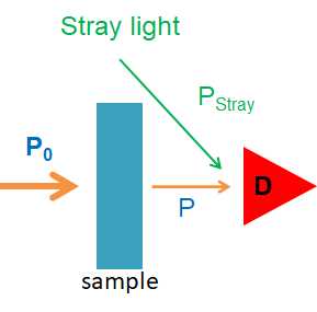
Stray radiation is the second contribution to instrumental deviations from Beer’s law. Stray radiation arises from imperfections in the wavelength selector that allow light to enter the instrument and to reach the detector without passing through the sample. As shown in Figure 8.2.4, stray radiation adds an additional contribution, P_stray, to the radiant power that reaches the detector

Figure\(\PageIndex{4}\): A simple illustration showing stray light,  whether not of the correct wavelength or not passing though the sample striking the detector.

Thus

\[A=-\log \frac{P_{\mathrm{T}}+P_{\text { stray }}}{P_{0}+P_{\text { stray }}} \nonumber\]

For a small concentration of analyte, P_stray is significantly smaller than P₀ and P_T, and the absorbance is unaffected by the stray radiation. For higher concentrations of analyte, less light passes through the sample and P_T and P_stray become similar in magnitude. This results is an absorbance that is smaller than expected, and a negative deviation from Beer’s law.