13.11: Time-Dependent Perturbation Theory

Time-independent perturbation theory is one of two categories of perturbation theory, the other being time-dependent perturbation. In time-independent perturbation theory the perturbation Hamiltonian is static (i.e., possesses no time dependence). Time-independent perturbation theory was presented by Erwin Schrödinger in a 1926 paper,shortly after he produced his theories in wave mechanics. Time-dependent perturbation theory, developed by Paul Dirac, studies the effect of a time-dependent perturbation V(t) applied to a time-independent Hamiltonian $H_0$. Since the perturbed Hamiltonian is time-dependent, so are its energy levels and eigenstates. Thus, the goals of time-dependent perturbation theory are slightly different from time-independent perturbation theory, where one may be interested in the following quantities:

• The time-dependent expectation value of some observable A, for a given initial state.
• The time-dependent amplitudes of those quantum states that are energy eigenkets (eigenvectors) in the unperturbed system.

The first quantity is important because it gives rise to the classical result of a measurement performed on a macroscopic number of copies of the perturbed system. The second quantity looks at the time-dependent probability of occupation for each eigenstate. This is particularly useful in laser physics, where one is interested in the populations of different atomic states in a gas when a time-dependent electric field is applied. We will briefly examine the method behind Dirac's formulation of time-dependent perturbation theory. Choose an energy basis ${\displaystyle {|n\rangle }}$$| n \rangle$ for the unperturbed system. (We drop the (0) superscripts for the eigenstates, because it is not useful to speak of energy levels and eigenstates for the perturbed system.)

If the unperturbed system is in eigenstate $|j \rangle$ at time $t = 0$, its state at subsequent times varies only by a phase (this is the Schrödinger picture, where state vectors evolve in time and operators are constant)

$$|j(t)\rangle =e^{-iE_{j}t/\hbar }|j\rangle$$

Now, introduce a time-dependent perturbing Hamiltonian $H_1(t)$. The Hamiltonian of the perturbed system is

$$H=H_{0}+H_1(t)$$

Let $|\psi (t)\rangle$ denote the quantum state of the perturbed system at time $t$ and obeys the time-dependent Schrödinger equation,

$$H|\psi (t)\rangle =i\hbar {\dfrac {\partial }{\partial t}}|\psi (t)\rangle$$

The quantum state at each instant can be expressed as a linear combination of the complete eigenbasis of $| n \rangle$:

$$|\psi (t)\rangle =\sum _{n}c_{n}(t)e^{-iE_{n}t/\hbar }|n\rangle$$

where the $c_n(t)$ coefficients are to be determined complex functions of t which we will refer to as amplitudes

We have explicitly extracted the exponential phase factors $\exp(-iE_{n}t/\hbar)$ on the right hand side. This is only a matter of convention, and may be done without loss of generality. The reason we go to this trouble is that when the system starts in the state ${\displaystyle |j\rangle }$$|j\rangle$ and no perturbation is present, the amplitudes have the convenient property that, for all t, $c_j(t) = 1$ and $c_n(t) = 0$ if $n \neq j$.

The square of the absolute amplitude $c_n(t)$ is the probability that the system is in state $n$ at time $t$, since

$$|\psi (t)\rangle =\sum _{n}c_{n}(t)e^{-iE_{n}t/\hbar }|n\rangle$$

Plugging into the Schrödinger equation and using the fact that $\partial/ \partial t$ acts by a chain rule, one obtains

$$\sum _{n}\left(i\hbar {\dfrac {\partial c_{n}}{\partial t}}-c_{n}(t)V(t)\right)e^{-iE_{n}t/\hbar }|n\rangle =0~.$$

By resolving the identity in front of V, this can be reduced to a set of partial differential equations for the amplitudes,

$${\dfrac {\partial c_{n}}{\partial t}}={\dfrac {-i}{\hbar }}\sum _{k}\langle n|H_1(t)|k\rangle \,c_{k}(t)\,e^{-i(E_{k}-E_{n})t/\hbar }~.$$

The matrix elements of $H_1$ play a similar role as in time-independent perturbation theory, being proportional to the rate at which amplitudes are shifted between states. Note, however, that the direction of the shift is modified by the exponential phase factor. Over times much longer than the energy difference $E_k − E_n$, the phase winds around 0 several times. If the time-dependence of $H_1$ is sufficiently slow, this may cause the state amplitudes to oscillate (e.g., such oscillations are useful for managing radiative transitions in a laser).

Two-Level System

Consider the two level system (i.e. $n=1,2$)

$$| \psi \rangle = \sum_ {n=1,2} c_n(t) | n \rangle_o$$

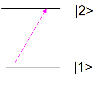
Solution of time-dependent perturbation for two level system:

$$i \hbar \dfrac{\partial c_1(t)}{\partial t} = c_1(t) H_{11}(t) + c_2 e^{-i \omega_o t} H_{12} (t)$$

$$i \hbar \dfrac{\partial c_2(t)}{\partial t} = c_2(t) H_{22}(t) + c_1 e^{+i \omega_o t} H_{21} (t)$$

where the matrix elements of the permutation (in terms of the eigenstates of $H(0)$) are

$$\langle m | H_1(t) | n \rangle = H_{mn}(t)$$

Assume initial state is $n=1$, and $H_{11}=H_{22}=0$

$$| \psi (t=0) \rangle = |1 \rangle$$

Probability of particle at $n=2$ at time $t$ after the perturbation is turned on (i.e., incident light):

$$c_2(t) = \dfrac{-i}{\hbar} \int_o^t e^{i \omega_o t} dt' H_{21}(t') \label{EQ1}$$

where

$$H_1(t) = \cos (\omega t) V(r)$$

$V(r)$ is an amplitude of polarization vector, which we can ignore for now.

If we assume incident frequency of incident light $\omega$ is comparable to the natural frequency of oscillation from $\omega _o$

$$\omega \approx \omega_o$$

then Equation $\ref{EQ1}$ can be simplified to

$$c_2(t) = - \dfrac{2i}{\hbar} \dfrac{\sin (\omega-\omega_o)t /2}{ (\omega-\omega_o )t} e^{i (\omega_0-\omega)t/2} H_{21}$$

Transition Probability

Assume initial state is $n=1$, and probability of transition from $n=1$ state to $n=2$ state is:

$$P_{12}(t) = | c_2(t) |^2 =\dfrac{4}{\hbar^2} | \dfrac{\sin (\omega-\omega_o)t /2}{ (\omega-\omega_o )t} |^2 | H_{21} |^2$$

What does this mean? Strangely, it means that the probability of makinga transition is actually oscillating sinusoidally (squared)! If you want to cause a transition, should turn off perturbation after time $\pi / |\omega- \omega_o|$or some odd multiple, when the system is in upper state with maximum probability.

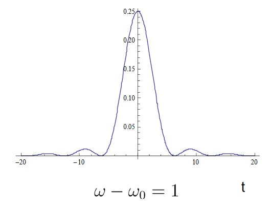
$P_{12}(t)$ is peaked at $\omega- \omega_o = 0$. The height of $|H_{12}t/2 \hbar |^2$ and width of $4\pi/t$ gets higher and narrower as time goes on. Recall this is perturbative treatment, however, and $P_{12}(t)$ cannot get bigger than 1, so perturbation theory breaks down eventually.

Contributors

• Wikipedia