
10.6: Butadiene is Stabilized by a Delocalization Energy
- Page ID
- 210875
\( \newcommand{\vecs}[1]{\overset { \scriptstyle \rightharpoonup} {\mathbf{#1}} } \)
\( \newcommand{\vecd}[1]{\overset{-\!-\!\rightharpoonup}{\vphantom{a}\smash {#1}}} \)
\( \newcommand{\id}{\mathrm{id}}\) \( \newcommand{\Span}{\mathrm{span}}\)
( \newcommand{\kernel}{\mathrm{null}\,}\) \( \newcommand{\range}{\mathrm{range}\,}\)
\( \newcommand{\RealPart}{\mathrm{Re}}\) \( \newcommand{\ImaginaryPart}{\mathrm{Im}}\)
\( \newcommand{\Argument}{\mathrm{Arg}}\) \( \newcommand{\norm}[1]{\| #1 \|}\)
\( \newcommand{\inner}[2]{\langle #1, #2 \rangle}\)
\( \newcommand{\Span}{\mathrm{span}}\)
\( \newcommand{\id}{\mathrm{id}}\)
\( \newcommand{\Span}{\mathrm{span}}\)
\( \newcommand{\kernel}{\mathrm{null}\,}\)
\( \newcommand{\range}{\mathrm{range}\,}\)
\( \newcommand{\RealPart}{\mathrm{Re}}\)
\( \newcommand{\ImaginaryPart}{\mathrm{Im}}\)
\( \newcommand{\Argument}{\mathrm{Arg}}\)
\( \newcommand{\norm}[1]{\| #1 \|}\)
\( \newcommand{\inner}[2]{\langle #1, #2 \rangle}\)
\( \newcommand{\Span}{\mathrm{span}}\) \( \newcommand{\AA}{\unicode[.8,0]{x212B}}\)
\( \newcommand{\vectorA}[1]{\vec{#1}} % arrow\)
\( \newcommand{\vectorAt}[1]{\vec{\text{#1}}} % arrow\)
\( \newcommand{\vectorB}[1]{\overset { \scriptstyle \rightharpoonup} {\mathbf{#1}} } \)
\( \newcommand{\vectorC}[1]{\textbf{#1}} \)
\( \newcommand{\vectorD}[1]{\overrightarrow{#1}} \)
\( \newcommand{\vectorDt}[1]{\overrightarrow{\text{#1}}} \)
\( \newcommand{\vectE}[1]{\overset{-\!-\!\rightharpoonup}{\vphantom{a}\smash{\mathbf {#1}}}} \)
\( \newcommand{\vecs}[1]{\overset { \scriptstyle \rightharpoonup} {\mathbf{#1}} } \)
\( \newcommand{\vecd}[1]{\overset{-\!-\!\rightharpoonup}{\vphantom{a}\smash {#1}}} \)
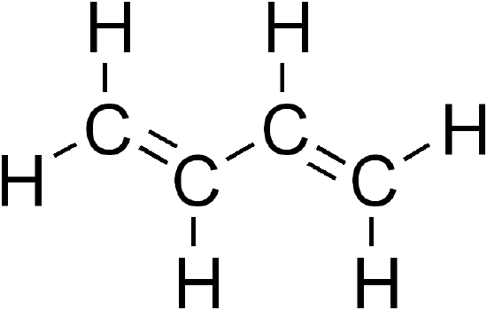
\(\newcommand{\avec}{\mathbf a}\) \(\newcommand{\bvec}{\mathbf b}\) \(\newcommand{\cvec}{\mathbf c}\) \(\newcommand{\dvec}{\mathbf d}\) \(\newcommand{\dtil}{\widetilde{\mathbf d}}\) \(\newcommand{\evec}{\mathbf e}\) \(\newcommand{\fvec}{\mathbf f}\) \(\newcommand{\nvec}{\mathbf n}\) \(\newcommand{\pvec}{\mathbf p}\) \(\newcommand{\qvec}{\mathbf q}\) \(\newcommand{\svec}{\mathbf s}\) \(\newcommand{\tvec}{\mathbf t}\) \(\newcommand{\uvec}{\mathbf u}\) \(\newcommand{\vvec}{\mathbf v}\) \(\newcommand{\wvec}{\mathbf w}\) \(\newcommand{\xvec}{\mathbf x}\) \(\newcommand{\yvec}{\mathbf y}\) \(\newcommand{\zvec}{\mathbf z}\) \(\newcommand{\rvec}{\mathbf r}\) \(\newcommand{\mvec}{\mathbf m}\) \(\newcommand{\zerovec}{\mathbf 0}\) \(\newcommand{\onevec}{\mathbf 1}\) \(\newcommand{\real}{\mathbb R}\) \(\newcommand{\twovec}[2]{\left[\begin{array}{r}#1 \\ #2 \end{array}\right]}\) \(\newcommand{\ctwovec}[2]{\left[\begin{array}{c}#1 \\ #2 \end{array}\right]}\) \(\newcommand{\threevec}[3]{\left[\begin{array}{r}#1 \\ #2 \\ #3 \end{array}\right]}\) \(\newcommand{\cthreevec}[3]{\left[\begin{array}{c}#1 \\ #2 \\ #3 \end{array}\right]}\) \(\newcommand{\fourvec}[4]{\left[\begin{array}{r}#1 \\ #2 \\ #3 \\ #4 \end{array}\right]}\) \(\newcommand{\cfourvec}[4]{\left[\begin{array}{c}#1 \\ #2 \\ #3 \\ #4 \end{array}\right]}\) \(\newcommand{\fivevec}[5]{\left[\begin{array}{r}#1 \\ #2 \\ #3 \\ #4 \\ #5 \\ \end{array}\right]}\) \(\newcommand{\cfivevec}[5]{\left[\begin{array}{c}#1 \\ #2 \\ #3 \\ #4 \\ #5 \\ \end{array}\right]}\) \(\newcommand{\mattwo}[4]{\left[\begin{array}{rr}#1 \amp #2 \\ #3 \amp #4 \\ \end{array}\right]}\) \(\newcommand{\laspan}[1]{\text{Span}\{#1\}}\) \(\newcommand{\bcal}{\cal B}\) \(\newcommand{\ccal}{\cal C}\) \(\newcommand{\scal}{\cal S}\) \(\newcommand{\wcal}{\cal W}\) \(\newcommand{\ecal}{\cal E}\) \(\newcommand{\coords}[2]{\left\{#1\right\}_{#2}}\) \(\newcommand{\gray}[1]{\color{gray}{#1}}\) \(\newcommand{\lgray}[1]{\color{lightgray}{#1}}\) \(\newcommand{\rank}{\operatorname{rank}}\) \(\newcommand{\row}{\text{Row}}\) \(\newcommand{\col}{\text{Col}}\) \(\renewcommand{\row}{\text{Row}}\) \(\newcommand{\nul}{\text{Nul}}\) \(\newcommand{\var}{\text{Var}}\) \(\newcommand{\corr}{\text{corr}}\) \(\newcommand{\len}[1]{\left|#1\right|}\) \(\newcommand{\bbar}{\overline{\bvec}}\) \(\newcommand{\bhat}{\widehat{\bvec}}\) \(\newcommand{\bperp}{\bvec^\perp}\) \(\newcommand{\xhat}{\widehat{\xvec}}\) \(\newcommand{\vhat}{\widehat{\vvec}}\) \(\newcommand{\uhat}{\widehat{\uvec}}\) \(\newcommand{\what}{\widehat{\wvec}}\) \(\newcommand{\Sighat}{\widehat{\Sigma}}\) \(\newcommand{\lt}{<}\) \(\newcommand{\gt}{>}\) \(\newcommand{\amp}{&}\) \(\definecolor{fillinmathshade}{gray}{0.9}\)1,3-Butadiene is a simple conjugated diene with the formula \(C_4H_6\) and can be viewed structurally as two vinyl groups (\(CH_2=CH_2\)) joined together with a single bond. Butadiene can occupy either a cis or trans conformers and at room temperature, 96% of butadiene exists as the trans conformer, which is 2.3 kcal/mole more stable than the cis structure.
For the simple application of applying Hückel theory for understanding the electronic structure of butadiene, we will ignore the energetic differences between the two conformers. As discussed previously, the molecular orbitals are linear combination of the 4 \(|p \rangle\) atomic orbitals at on the carbon atoms:
\[|\Psi_i \rangle = \sum_i^4 c_{ij} |p_{i} \rangle \]
or explicitly
\[|\Psi_i \rangle =c_{i1} |p_1 \rangle+ c_ {i2} | p_2 \rangle + c_ {i3} | p_3 \rangle + c_ {i4} | p_4 \rangle \label{general}\]
for the ith molecular orbital \(|\Psi_i \rangle \). The secular equations that need to be solved are
\[\begin{bmatrix} H_{11} - ES_{11} & H_{12} - ES_{12} & H_{13} - ES_{13} & H_{14} - ES_{14} \\ H_{12} - ES_{12} & H_{22} - ES_{22} & H_{23} - ES_{23} & H_{24} - ES_{24} \\ H_{13} - ES_{13} & H_{23} - ES_{23} & H_{33} - ES_{33} & H_{34} - ES_{34} \\ H_{14} - ES_{14} & H_{24} - ES_{24} & H_{34} - ES_{34} & H_{44} - ES_{44} \\ \end{bmatrix} \times\begin{bmatrix} c_1 \\ c_2 \\ c_3 \\ c_4 \\ \end{bmatrix}= 0 \label{complete}\]
If the standard Hückel theory approximations were used
\[ H_{ii}- ES_{ii} = \alpha\]
and
\[ H_{ij}- ES_{ij} = \beta\]
when \(i=j\pm 1\), otherwise
\[ H_{ij}- ES_{ij} = 0\]
then the secular equations for butadience in Equation \(\ref{complete}\) become
\[\begin{bmatrix} \alpha - E & \beta & 0 & 0 \\ \beta & \alpha - E & \beta & 0 \\ 0 & \beta & \alpha - E & \beta \\ 0 & 0 & \beta & \alpha - E \\ \end{bmatrix} \times\begin{bmatrix} c_1 \\ c_2 \\ c_3 \\ c_4 \\ \end{bmatrix}= 0 \label{Huckel1}\]
Solving Equation \(\ref{Huckel1}\) for \(\{c_i\}\) coefficients and energy secular equation requires extracting the roots of the secular determinant:
\[\left|\begin{array}{cccc}\alpha-E&\beta&0&0\\\beta&\alpha-E&\beta&0\\0&\beta&\alpha-E&\beta\\0&0&\beta&\alpha-E\end{array}\right|=0\label{24}\]
If both sides of Equation \(\ref{24}\) were divided by \(\beta^{4}\) and a new variable \(x\) is defined
\[x=\dfrac{\alpha-E}{\beta}\label{25}\]
then Equation \(\ref{24}\) simplifies further to
\[\left|\begin{array}{cccc}x&1&0&0\\1&x&1&0\\0&1&x&1\\0&0&1&x\end{array}\right|=0\label{26}\]
This is essentially the connection matrix for the butadiene molecule. Each pair of connected atoms is represented by 1, each non-connected pair by 0 and each diagonal element by \(x\). Expansion of the determinant in Equation \(\ref{26}\) gives the 4th order polynomial equation
\[x^{4}-3x^{2}+1=0 \label{27}\]
While solving 4th order equations typically require numerical estimation, Equation \(\ref{27}\) can be further simplified by recognizing that it is a quadratic equation in terms of \(x^{2}\). Therefore, the roots are
\[x^{2}= \dfrac{3\pm\sqrt{5}}{2}\]
or \(x=\pm\; 0.618\) and \(x= \pm\; 1.618\). Since \(\alpha\) and \(\beta\) are negative, these molecular orbital energies can ordered in terms of energy (from lowest to highest):
\[E_1=\alpha+1.618\beta \label{E1}\]
\[E_2=\alpha+0.618\beta \label{E2} \]
\[E_3=\alpha-0.618\beta \label{E3} \]
\[E_4=\alpha-1.618\beta \label{E4} \]
This sequence of energies is displayed in the energy diagram of Figure \(\PageIndex{1}\).
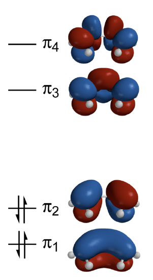
Each p atomic orbital of carbon contributes a single electron to the \(\pi\) manifold, so the ground-state occupation of the resulting four \(\pi\) electrons have a \(\pi_1^{2}\pi_2^{2}\) configuration (Figure \(\PageIndex{1}\)). The the total \(\pi\)-electron energy is then determined by adding up the energies in Equations \(\ref{E1}\)-\(\ref{E4}\) and scaling by their occupations to get
\[E_{\pi} (butadiene) =2(\alpha+1.618\beta)+2(\alpha+0.618\beta)=4\alpha + 4.472\beta \label{29}\]
If butadiene were described as two localized double bond (as in its dominant valence-bond structure), then its \(\pi\)-electron energy would be given by twice the \(E_{\pi}\) predicted for the ethlyene molecule:
\[2 \times E_{\pi} (ethylene)=2 \times 2(\alpha+\beta) = 4\alpha + 4\beta \label{30}\]
Comparing Equation \(\ref{29}\) with Equation \(\ref{29}\), the total \(\pi\) energy of butadiene lies lower than the total \(\pi\) energy of two double bonds by \(0.48\beta\) (the \(\sigma\) bond does not contribute). This difference is known as the delocalization energy; a typical estimate of \(\beta\) is around -75 kJ/mol, which results in a delocalization energy for butadiene of -35 kJ/mol.
The delocalization energy is the extra stabilization resulting from the electrons extending over the whole molecule.
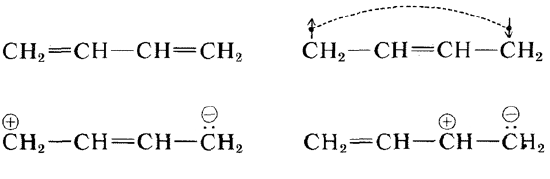
Delocalization energy is intrinsic to molecular orbital theory, since it results from breaking the two-center bond concept with the molecular orbitals that spread over more that just one pair of atoms. However, within the two-center theory of valence bond theory, the delocalization energy results from a stabilization energy attributed to resonance. Several conventional valence bond resonance structures that can be written for 1,3-butadiene, four of which are shown in Figure \(\PageIndex{2}\). However, while structure \(2a\) dominates, the other resonance structures also contribute to describing the total molecule and hence predict a corresponding stabilization energy akin to the delocalization energy in molecular orbital theory.
In general, the true description of the bonidng within the valence bond theory is a superposition of resonance structures with amplitudes that are determined via a variational optimization to find the lowest possible energy for the valence bond wavefunctions.
The solving the secular equations also gives the \(\{c_{ij}\}\) coefficients for the molecular orbitals in Equation \(\ref{general}\) (not demonstrated):
\[|\Psi_1 \rangle =0.37 |p_1 \rangle + 0.60 | p_2 \rangle + 0.60 | p_3 \rangle + 0.37 | p_4 \rangle \label{MO1}\]
\[|\Psi_3 \rangle =0.60 |p_1 \rangle + 0.37 | p_2 \rangle -0.37 | p_3 \rangle - 0.60 | p_4 \rangle \label{MO2}\]
\[|\Psi_3 \rangle =0.60 |p_1 \rangle - 0.37 | p_2 \rangle -0.37 | p_3 \rangle + 0.60 | p_4 \rangle \label{MO3}\]
\[|\Psi_4 \rangle =0.37 |p_1 \rangle - 0.60 | p_2 \rangle + 0.60 | p_3 \rangle - 0.37 | p_4 \rangle \label{MO4}\]
These are depicted in Figure \(\PageIndex{3}\).
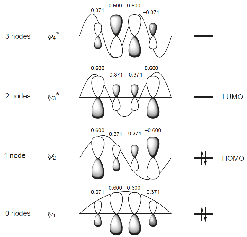
Not the correlation of the energy of the wavefunctions to the number of nodes in the wavefunction; this is the general trend observed in previous systems like the particles in the box and atomic orbitals. The four 3-D calculated molecular orbitals are contrasted in Figure \(\PageIndex{1}\):
Aromaticity in Benzene
Aromatic systems provide the most significant applications of Hückel theory. For benzene, we find the secular equation
\[\left|\begin{array}{cccccc}x&1&0&0&0&1\\1&x&1&0&0&0\\0&1&x&1&0&0\\0&0&1&x&1&0\\0&0&0&1&x&1\\1&0&0&0&1&x\end{array}\right|=0\label{31}\]
with the six roots \(x=\pm2,\pm1,\pm1\). The energy levels are \(E=\alpha\pm2\beta\) and two-fold degenerate \(E=\alpha\pm\beta\). With the three lowest MO's occupied, we have
\[E_{\pi}=2(\alpha+2\beta)+4(\alpha+\beta)=6\alpha+8\beta\label{32}\]
Since the energy of three localized double bonds is \(6\alpha+6\beta\), the delocalization energy equals \(2\beta\). The thermochemical value is -152 kJmol-1.
Contributors
- Wikipedia
- Anonymous