6.2: The Wavefunctions of a Rigid Rotator are Called Spherical Harmonics

The solutions to the hydrogen atom Schrödinger equation are functions that are products of a spherical harmonic functions and a radial function.

\[ \psi _{n, l, m_l } (r, \theta , \phi) = R_{n,l} (r) Y^{m_l}_l (\theta , \phi) \label {6.2.20}\]

The wavefunctions for the hydrogen atom depend upon the three variables r, \(\theta\), and \(\phi \) and the three quantum numbers n, \(l\), and \(m_l\). The variables give the position of the electron relative to the proton in spherical coordinates. The absolute square of the wavefunction, \(| \psi (r, \theta , \phi )|^2\), evaluated at \(r\), \(\theta \), and \(\phi\) gives the probability density of finding the electron inside a differential volume \(d \tau\), centered at the position specified by \(r\), \(\theta \), and \(\phi\).

Exercise \(\PageIndex{1}\)

What is the value of the integral

\[ \int \limits _{ all space} | \psi (r, \theta , \phi )|^2 d \tau \nonumber\]

or in braket notation

\[\langle \psi (r, \theta , \phi ) | \psi (r, \theta , \phi ) \rangle \;? \nonumber\]

The quantum numbers have names:

• \(n\) is called the principle quantum number,
• \(l\) is called the angular momentum quantum number, and
• \(m_l\) is called the magnetic quantum number because (as we will see, the energy in a magnetic field depends upon \(m_l\)).

Often \(l\) is called the azimuthal quantum number because it is a consequence of the \(\theta\)-equation, which involves the azimuthal angle \(\Theta \), referring to the angle to the zenith. These quantum numbers have specific values that are dictated by the physical constraints or boundary conditions imposed upon the Schrödinger equation: n must be an integer greater than 0, \(l\) can have the values 0 to n‑1, and \(m_l\) can have \(2l + 1\) values ranging from \(-l\) ‑ to \(+l\) in unit or integer steps.

The values of the quantum number \(l\) usually are coded by a letter: s means 0, p means 1, d means 2, f means 3; the next codes continue alphabetically (e.g., g means \(l = 4\)). The quantum numbers specify the quantization of physical quantities. The discrete energies of different states of the hydrogen atom are given by n, the magnitude of the angular momentum is given by \(l\), and one component of the angular momentum (usually chosen by chemists to be the z‑component) is given by \(m_l\). The total number of orbitals with a particular value of \(n\) is \(n^2\).

The \(\Phi\) function is found to have the quantum number \(m\), where

\[\Phi_m (\phi) = A_m e^{im\phi}\]

and \(A_m\) is the normalization constant and \(m = 0, \pm1, \pm2 ... \pm\infty\). The \(\Theta\) function was solved and is known as Legendre polynomials, which have quantum numbers \(m\) and \(\ell\). When \(\Theta\) and \(\Phi\) are multiplied together, the product is known as spherical harmonics with labeling \(Y_{J}^{m} (\theta, \phi)\).

Figure \(\PageIndex{1}\): Spherical Harmonics as commonly displayed, sorted by increasing energies and aligned for symmetry.

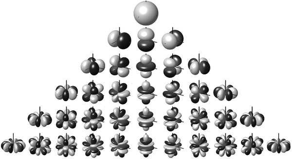
Figure \(\PageIndex{1}\) shows the spherical harmonics \(Y_J^M\), which are solutions of the angular Schrödinger equation of a 3D rigid rotor. These are explicitly written in Table \(\PageIndex{1}\). Notice that these functions are complex in nature.

Table \(\PageIndex{1}\): spherical harmonics \(Y_J^M\)

\(m_J\)	\(J\)	\(\Theta ^{m_J}_J (\theta)\)	\(\Phi (\varphi)\)	\(Y^{m_J}_J (\theta , \varphi)\)
0	0	\(\dfrac {1}{\sqrt {2}}\)	\(\dfrac {1}{\sqrt {2 \pi}}\)	\(\dfrac {1}{\sqrt {4 \pi}}\)
0	1	\(\sqrt {\dfrac {3}{2}}\cos \theta\)	\(\dfrac {1}{\sqrt {2 \pi}}\)	\(\sqrt {\dfrac {3}{4 \pi}}\cos \theta\)
1	1	\(\sqrt {\dfrac {3}{4}}\sin \theta\)	\(\dfrac {1}{\sqrt {2 \pi}}e^{i \varphi}\)	\(\sqrt {\dfrac {3}{8 \pi}}\sin \theta e^{i \varphi}\)
-1	1	\(\sqrt {\dfrac {3}{4}}\sin \theta\)	\(\dfrac {1}{\sqrt {2 \pi}}e^{-i\varphi}\)	\(\sqrt {\dfrac {3}{8 \pi}}\sin \theta e^{-i \varphi}\)
0	2	\(\sqrt {\dfrac {5}{8}}(3\cos ^2 \theta - 1)\)	\(\dfrac {1}{\sqrt {2 \pi}}\)	\(\sqrt {\dfrac {5}{16\pi}}(3\cos ^2 \theta - 1)\)
1	2	\(\sqrt {\dfrac {15}{4}} \sin \theta \cos \theta \)	\(\dfrac {1}{\sqrt {2 \pi}}e^{i \varphi}\)	\(\sqrt {\dfrac {15}{8\pi}} \sin \theta \cos \theta e^{i\varphi}\)
-1	2	\(\sqrt {\dfrac {15}{4}} \sin \theta \cos \theta \)	\(\dfrac {1}{\sqrt {2 \pi}}e^{-i\varphi}\)	\(\sqrt {\dfrac {15}{8\pi}} \sin \theta \cos \theta e^{-i\varphi}\)
2	2	\(\sqrt {\dfrac {15}{16}} \sin ^2 \theta \)	\(\dfrac {1}{\sqrt {2 \pi}}e^{2i\varphi}\)	\(\sqrt {\dfrac {15}{32\pi}} \sin ^2 \theta e^{2i\varphi} \)
-2	2	\(\sqrt {\dfrac {15}{16}} \sin ^2 \theta \)	\(\dfrac {1}{\sqrt {2 \pi}}e^{-2i\varphi}\)	\(\sqrt {\dfrac {15}{32\pi}} \sin ^2 \theta e^{-2i\varphi} \)

Exercise \(\PageIndex{2}\)

Consider several values for \(n\), and show that the number of orbitals for each \(n\) is \(n^2\).

Exercise \(\PageIndex{3}\)

Construct a table summarizing the allowed values for the quantum numbers \(n\), \(l\), and \(m_l\). for energy levels 1 through 7 of hydrogen.

Exercise \(\PageIndex{4}\)

The notation 3d specifies the quantum numbers for an electron in the hydrogen atom. What are the values for \(n\) and \(l\)? What are the values for the energy and angular momentum? What are the possible values for the magnetic quantum number? What are the possible orientations for the angular momentum vector?

The hydrogen atom wavefunctions, \(\psi (r, \theta , \phi )\), are called atomic orbitals. An atomic orbital is a function that describes one electron in an atom. The wavefunction with \(n = 1\), \(\ell\) = 0\), (\(m_ell=0\) is called the 1s orbital, and an electron that is described by this function is said to be “in” the ls orbital, i.e. have a 1s orbital state. The constraints on \(n\), \(\ell\), and \(m_\ell\) that are imposed during the solution of the hydrogen atom Schrödinger equation explain why there is a single 1s orbital, why there are three 2p orbitals, five 3d orbitals, etc. We will see when we consider multi-electron atoms, these constraints explain the features of the Periodic Table. In other words, the Periodic Table is a manifestation of the Schrödinger model and the physical constraints imposed to obtain the solutions to the Schrödinger equation for the hydrogen atom.

Visualizing the variation of an electronic wavefunction with \(r\), \(\theta\), and \(\phi\) is important because the absolute square of the wavefunction depicts the charge distribution (electron probability density) in an atom or molecule. The charge distribution is central to chemistry because it is related to chemical reactivity. For example, an electron-deficient part of one molecule is attracted to an electron-rich region of another molecule, and such interactions play a major role in chemical interactions ranging from substitution and addition reactions to protein folding and the interaction of substrates with enzymes.

Visualizing wavefunctions and charge distributions is challenging because it requires examining the behavior of a function of three variables in three-dimensional space. This visualization is made easier by considering the radial and angular parts separately, but plotting the radial and angular parts separately do not reveal the shape of an orbital very well. The shape can be revealed better in a probability density plot. To make such a three-dimensional plot, divide space up into small volume elements, calculate \(\psi^* \psi \) at the center of each volume element, and then shade, stipple or color that volume element in proportion to the magnitude of \(\psi^* \psi \). Do not confuse such plots with polar plots, which look similar. Probability densities also can be represented by contour maps, as shown in Figure \(\PageIndex{2}\).

Figure \(\PageIndex{2}\): Contour plots in the x-y plane for the \(2p_x\) and \(3p_x\) orbitals of the hydrogen atom. The plots map lines of constant values of \(R(r)^2\); red lines follow paths of high \(R(r)^2\), blue for low \(R(r)^2\). The angular function used to create the figure was a linear combination of two Spherical Harmonic functions.

Methods for separately examining the radial portions of atomic orbitals provide useful information about the distribution of charge density within the orbitals. Graphs of the radial functions, \(R(r)\), for the 1s, 2s, and 2p orbitals plotted in Figure \(\PageIndex{3}\).

Figure \(\PageIndex{3}\): Radial function, \(R(r)\), for the 1s, 2s, and 2p orbitals.

The 1s function in Figure \(\PageIndex{3}\) starts with a high positive value at the nucleus and exponentially decays to essentially zero after 5 Bohr radii. The high value at the nucleus may be surprising, but as we shall see later, the probability of finding an electron at the nucleus is vanishingly small.

Next notice how the radial function for the 2s orbital, Figure \(\PageIndex{3}\), goes to zero and becomes negative. This behavior reveals the presence of a radial node in the function. A radial node occurs when the radial function equals zero other than at \(r = 0\) or \(r = ∞\). Nodes and limiting behaviors of atomic orbital functions are both useful in identifying which orbital is being described by which wavefunction. For example, all of the s functions have non-zero wavefunction values at \(r = 0\), but p, d, f and all other functions go to zero at the origin. It is useful to remember that there are \(n-1-l\) radial nodes in a wavefunction, which means that a 1s orbital has no radial nodes, a 2s has one radial node, and so on.

Exercise \(\PageIndex{5}\)

Examine the mathematical forms of the radial wavefunctions. What feature in the functions causes some of them to go to zero at the origin while the s functions do not go to zero at the origin?

Exercise \(\PageIndex{6}\)

What mathematical feature of each of the radial functions controls the number of radial nodes?

Answer

The Laguerre polynomial controls the radial nodes with the number of roots for the Laguerre polynomial is the number of radial nodes.

Exercise \(\PageIndex{7}\)

At what value of \(r\) does the 2s radial node occur?

Answer

A node exists when the radial portion of the wavefunction equals 0. The radial portion of the 2s wavefunction is:

\[\left(\frac{1}{2 \sqrt{2}}\right)\left(\frac{Z}{\alpha_{0}}\right)^{\frac{3}{2}}(2-\rho) e^{\frac{-\rho}{2}}\]

where

\[\rho=\frac{Z r}{\alpha_{0}}\]

\*Z=1\( for the hydrogen atom

and \(\alpha_{0}=$\) is the Bohr radius

Therefore:

\[\left(\frac{1}{2 \sqrt{2}}\right)\left(\frac{1}{\alpha_{0}}\right)^{\frac{3}{2}}\left(2-\frac{r}{\alpha_{0}}\right) e^{\frac{-2 r}{\alpha_{0}}}\]

For this wavefunction,

• \(\left(\frac{1}{\alpha_{0}}\right)^{\frac{3}{2}}\) is a constant and will never equal 0.
• \(e^{\frac{-2 r}{\alpha_{0}}}\) is an exponential, and will also never equal 0.

Therefore, our node is when \(\left(2-\frac{r}{\alpha_{0}}\right)=0\) and \[r=2 \alpha_{0}\]

Exercise \(\PageIndex{8}\)

Make a table that provides the energy, number of radial nodes, and the number of angular nodes and total number of nodes for each function with \(n = 1\), \(n=2\), and \(n=3\). Identify the relationship between the energy and the number of nodes. Identify the relationship between the number of radial nodes and the number of angular nodes.

Answer

Wavefunction	Energy	Total Nodes	Radial Nodes	Angular Nodes
1s	13.6 eV	0	0	0
2s	3.4 eV	1	1	0
2p	3.4 eV	1	0	1
3s	1.5 eV	2	2	0
3p	1.5 eV	2	1	1
3d	1.5 eV	2	0	2

The energy of the electron in each wavefunction is \[E = \dfrac{Z^2E_h}{2n^2}\]

The number of total nodes is (N-1\), the number of radial nodes is \(N-L-1\) and the number of angular nodes is \(L\).

The quantity \(R(r)^* R(r)\) gives the radial probability density; i.e., the probability density for the electron to be at a point located the distance \(r\) from the proton. Radial probability densities for three atomic orbitals are plotted in Figure \(\PageIndex{4}\).

Figure \(\PageIndex{4}\): Radial probability densities for the 1s, 2s, and 2p orbitals.

When the radial probability density for every value of \(r\) is multiplied by the area of the spherical surface represented by that particular value of r, we get the radial distribution function. The radial distribution function gives the probability density for an electron to be found anywhere on the surface of a sphere located a distance r from the proton. Since the area of a spherical surface is \(4 \pi r^2\), the radial distribution function is given by

\[\underbrace{4 \pi r^2 R(r) ^* R(r)}_{radial probability density}\]

Radial distribution functions are shown in Figure \(\PageIndex{5}\). At small values of \(r\), the radial distribution function is low because the small surface area for small radii modulates the high value of the radial probability density function near the nucleus. As we increase \(r\), the surface area associated with a given value of r increases, and the \(r^2\) term causes the radial distribution function to increase even though the radial probability density is beginning to decrease. At large values of \(r\), the exponential decay of the radial function outweighs the increase caused by the \(r^2\) term and the radial distribution function decreases.

Figure \(\PageIndex{5}\): The radial distribution function for the 1s, 2s, and 2p orbitals.

Exercise \(\PageIndex{9}\)

Write a quality comparison of the radial function and radial distribution function for the 2s orbital. See Figure \(\PageIndex{6}\).

Answer

\(\4pi R(r)^2 R(r)^2\) gives the radial probability density of the distance of electron at distance r from the nucleus.

The radial probability function is low at small values of \(r\) because of a small surface area near nucleus, for example at 2s at a small value of r the radial probability function is low.

At higher values of r the surface area increases while radial probability density decreases, this causes the radial distribution function to increase.

In contrast the radial probability density is high at small surface area and when r is near the nucleus, i.e low values of r.

Figure \(\PageIndex{6}\): Comparison of a) the radial distribution function and b) the radial probability density for the 2s orbital.

Contributors

• David M. Hanson, Erica Harvey, Robert Sweeney, Theresa Julia Zielinski ("Quantum States of Atoms and Molecules")