
5.9: The Rigid Rotator is a Model for a Rotating Diatomic Molecule
- Page ID
- 210820
\( \newcommand{\vecs}[1]{\overset { \scriptstyle \rightharpoonup} {\mathbf{#1}} } \)
\( \newcommand{\vecd}[1]{\overset{-\!-\!\rightharpoonup}{\vphantom{a}\smash {#1}}} \)
\( \newcommand{\id}{\mathrm{id}}\) \( \newcommand{\Span}{\mathrm{span}}\)
( \newcommand{\kernel}{\mathrm{null}\,}\) \( \newcommand{\range}{\mathrm{range}\,}\)
\( \newcommand{\RealPart}{\mathrm{Re}}\) \( \newcommand{\ImaginaryPart}{\mathrm{Im}}\)
\( \newcommand{\Argument}{\mathrm{Arg}}\) \( \newcommand{\norm}[1]{\| #1 \|}\)
\( \newcommand{\inner}[2]{\langle #1, #2 \rangle}\)
\( \newcommand{\Span}{\mathrm{span}}\)
\( \newcommand{\id}{\mathrm{id}}\)
\( \newcommand{\Span}{\mathrm{span}}\)
\( \newcommand{\kernel}{\mathrm{null}\,}\)
\( \newcommand{\range}{\mathrm{range}\,}\)
\( \newcommand{\RealPart}{\mathrm{Re}}\)
\( \newcommand{\ImaginaryPart}{\mathrm{Im}}\)
\( \newcommand{\Argument}{\mathrm{Arg}}\)
\( \newcommand{\norm}[1]{\| #1 \|}\)
\( \newcommand{\inner}[2]{\langle #1, #2 \rangle}\)
\( \newcommand{\Span}{\mathrm{span}}\) \( \newcommand{\AA}{\unicode[.8,0]{x212B}}\)
\( \newcommand{\vectorA}[1]{\vec{#1}} % arrow\)
\( \newcommand{\vectorAt}[1]{\vec{\text{#1}}} % arrow\)
\( \newcommand{\vectorB}[1]{\overset { \scriptstyle \rightharpoonup} {\mathbf{#1}} } \)
\( \newcommand{\vectorC}[1]{\textbf{#1}} \)
\( \newcommand{\vectorD}[1]{\overrightarrow{#1}} \)
\( \newcommand{\vectorDt}[1]{\overrightarrow{\text{#1}}} \)
\( \newcommand{\vectE}[1]{\overset{-\!-\!\rightharpoonup}{\vphantom{a}\smash{\mathbf {#1}}}} \)
\( \newcommand{\vecs}[1]{\overset { \scriptstyle \rightharpoonup} {\mathbf{#1}} } \)
\( \newcommand{\vecd}[1]{\overset{-\!-\!\rightharpoonup}{\vphantom{a}\smash {#1}}} \)
\(\newcommand{\avec}{\mathbf a}\) \(\newcommand{\bvec}{\mathbf b}\) \(\newcommand{\cvec}{\mathbf c}\) \(\newcommand{\dvec}{\mathbf d}\) \(\newcommand{\dtil}{\widetilde{\mathbf d}}\) \(\newcommand{\evec}{\mathbf e}\) \(\newcommand{\fvec}{\mathbf f}\) \(\newcommand{\nvec}{\mathbf n}\) \(\newcommand{\pvec}{\mathbf p}\) \(\newcommand{\qvec}{\mathbf q}\) \(\newcommand{\svec}{\mathbf s}\) \(\newcommand{\tvec}{\mathbf t}\) \(\newcommand{\uvec}{\mathbf u}\) \(\newcommand{\vvec}{\mathbf v}\) \(\newcommand{\wvec}{\mathbf w}\) \(\newcommand{\xvec}{\mathbf x}\) \(\newcommand{\yvec}{\mathbf y}\) \(\newcommand{\zvec}{\mathbf z}\) \(\newcommand{\rvec}{\mathbf r}\) \(\newcommand{\mvec}{\mathbf m}\) \(\newcommand{\zerovec}{\mathbf 0}\) \(\newcommand{\onevec}{\mathbf 1}\) \(\newcommand{\real}{\mathbb R}\) \(\newcommand{\twovec}[2]{\left[\begin{array}{r}#1 \\ #2 \end{array}\right]}\) \(\newcommand{\ctwovec}[2]{\left[\begin{array}{c}#1 \\ #2 \end{array}\right]}\) \(\newcommand{\threevec}[3]{\left[\begin{array}{r}#1 \\ #2 \\ #3 \end{array}\right]}\) \(\newcommand{\cthreevec}[3]{\left[\begin{array}{c}#1 \\ #2 \\ #3 \end{array}\right]}\) \(\newcommand{\fourvec}[4]{\left[\begin{array}{r}#1 \\ #2 \\ #3 \\ #4 \end{array}\right]}\) \(\newcommand{\cfourvec}[4]{\left[\begin{array}{c}#1 \\ #2 \\ #3 \\ #4 \end{array}\right]}\) \(\newcommand{\fivevec}[5]{\left[\begin{array}{r}#1 \\ #2 \\ #3 \\ #4 \\ #5 \\ \end{array}\right]}\) \(\newcommand{\cfivevec}[5]{\left[\begin{array}{c}#1 \\ #2 \\ #3 \\ #4 \\ #5 \\ \end{array}\right]}\) \(\newcommand{\mattwo}[4]{\left[\begin{array}{rr}#1 \amp #2 \\ #3 \amp #4 \\ \end{array}\right]}\) \(\newcommand{\laspan}[1]{\text{Span}\{#1\}}\) \(\newcommand{\bcal}{\cal B}\) \(\newcommand{\ccal}{\cal C}\) \(\newcommand{\scal}{\cal S}\) \(\newcommand{\wcal}{\cal W}\) \(\newcommand{\ecal}{\cal E}\) \(\newcommand{\coords}[2]{\left\{#1\right\}_{#2}}\) \(\newcommand{\gray}[1]{\color{gray}{#1}}\) \(\newcommand{\lgray}[1]{\color{lightgray}{#1}}\) \(\newcommand{\rank}{\operatorname{rank}}\) \(\newcommand{\row}{\text{Row}}\) \(\newcommand{\col}{\text{Col}}\) \(\renewcommand{\row}{\text{Row}}\) \(\newcommand{\nul}{\text{Nul}}\) \(\newcommand{\var}{\text{Var}}\) \(\newcommand{\corr}{\text{corr}}\) \(\newcommand{\len}[1]{\left|#1\right|}\) \(\newcommand{\bbar}{\overline{\bvec}}\) \(\newcommand{\bhat}{\widehat{\bvec}}\) \(\newcommand{\bperp}{\bvec^\perp}\) \(\newcommand{\xhat}{\widehat{\xvec}}\) \(\newcommand{\vhat}{\widehat{\vvec}}\) \(\newcommand{\uhat}{\widehat{\uvec}}\) \(\newcommand{\what}{\widehat{\wvec}}\) \(\newcommand{\Sighat}{\widehat{\Sigma}}\) \(\newcommand{\lt}{<}\) \(\newcommand{\gt}{>}\) \(\newcommand{\amp}{&}\) \(\definecolor{fillinmathshade}{gray}{0.9}\)To develop a description of the rotational states, we will consider the molecule to be a rigid object, i.e. the bond lengths are fixed and the molecule cannot vibrate. This model for rotation is called the rigid-rotor model. It is a good approximation (even though a molecule vibrates as it rotates, and the bonds are elastic rather than rigid) because the amplitude of the vibration is small compared to the bond length.
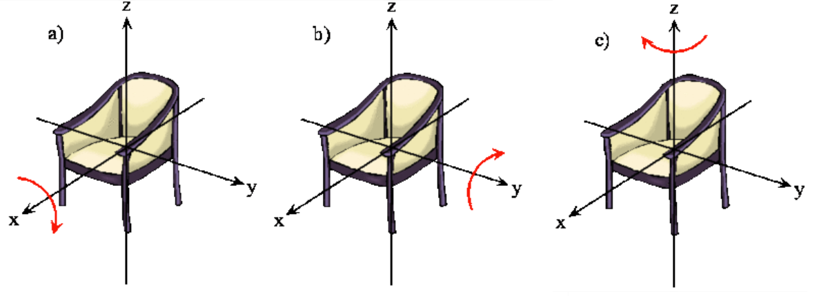
The rotation of a rigid object in space is very simple to visualize. Pick up any object and rotate it. There are orthogonal rotations about each of the three Cartesian coordinate axes just as there are orthogonal translations in each of the directions in three-dimensional space (Figures \(\PageIndex{1}\) and \(\PageIndex{2}\)). These rotations are said to be orthogonal because one can not describe a rotation about one axis in terms of rotations about the other axes just as one can not describe a translation along the x-axis in terms of translations along the y- and z-axes. For a linear molecule, the motion around the interatomic axis (x-axis) is not considered a rotation.
In this section we examine the rotational states for a diatomic molecule by comparing the classical interpretation of the angular momentum vector with the probabilistic interpretation of the angular momentum wavefunctions. We want to answer the following types of questions. How do we describe the orientation of a rotating diatomic molecule in space? Is the molecule actually rotating? What properties of the molecule can be physically observed? In what ways does the quantum mechanical description of a rotating molecule differ from the classical image of a rotating molecule?
Introduction to Microwave Spectroscopy
The permanent electric dipole moments of polar molecules can couple to the electric field of electromagnetic radiation. This coupling induces transitions between the rotational states of the molecules. The energies that are associated with these transitions are detected in the far infrared and microwave regions of the spectrum. For example, the microwave spectrum for carbon monoxide spans a frequency range of 100 to 1200 GHz, which corresponds to 3 - 40 \(cm^{-1}\).
The selection rules for the rotational transitions are derived from the transition moment integral by using the spherical harmonic functions and the appropriate dipole moment operator, \(\hat {\mu}\).
\[ \mu _T = \int Y_{J_f}^{m_f*} \hat {\mu} Y_{J_i}^{m_i} \sin \theta \,d \theta\, d \varphi \label{5.9.1a} \]
or in braket notation
\[\mu _T = \langle Y_{J_f}^{m_f} | \hat {\mu} | Y_{J_i}^{m_i} \rangle \label{5.9.1b}\]
Evaluating the transition moment integral involves a bit of mathematical effort. This evaluation reveals that the transition moment depends on the square of the dipole moment of the molecule, \(\mu ^2\) and the rotational quantum number, \(J\), of the initial state in the transition,
\[\mu _T = \mu ^2 \dfrac {J + 1}{2J + 1} \label {5.9.2}\]
and that the selection rules for rotational transitions are
\[\Delta J = \pm 1 \label {5.9.3}\]
and
\[\Delta m_J = 0, \pm 1 \label {5.9.4}\]
A photon is absorbed for \(\Delta J = +1\) and emitted for \(\Delta J = -1\).
Explain why your microwave oven heats water, but not air. Hint: draw and compare Lewis structures for components of air and for water.
The energies of the \(J^{th}\) rotational levels are given by
\[E_J = J(J + 1) \dfrac {\hbar ^2}{2I} \label{energy}\]
with each \(J^{th}\) energy level having a degeneracy of \(2J+1\) due to the different possible \(m_J\) values.
Each energy level of a rigid rotor has a degeneracy of \(2J+1\) due to the different \(m_J\) values.
Transition Energies
The transition energies for absorption of radiation are given by
\[\begin{align} E_{photon} &= \Delta E \\[4pt] &= E_f - E_i \\[4pt] &= h \nu \\[4pt] &= hc \bar {\nu} \label {5.9.5} \end{align}\]
Substituting the relationship for energy (Equation \ref{energy}) into Equation \ref{5.9.5} results in
\[h \nu =hc \bar {\nu} = J_f (J_f +1) \dfrac {\hbar ^2}{2I} - J_i (J_i +1) \dfrac {\hbar ^2}{2I} \label {5.9.6}\]
with \(J_i\) and \(J_f\) representing the rotational quantum numbers of the initial (lower) and final (upper) levels involved in the absorption transition.
Since microwave spectroscopists use frequency units and infrared spectroscopists use wavenumber units when describing rotational spectra and energy levels, both \(\nu\) and \(\bar {\nu}\) are included in Equation \(\ref{5.9.6}\). When we add in the constraints imposed by the selection rules, \(J_f\) can be replaced by \(J_i + 1\), because the selection rule requires \(J_f – J_i = 1\) for the absorption of a photon (Equation \ref{5.9.3}). The equation for absorption transitions (Equation \ref{5.9.6}) then can be written in terms of the only the quantum number \(J_i\) of the initial state.
\[\begin{align} E_{photon} &= h \nu \\[4pt] &= hc \bar {\nu} \\[4pt] &= 2 (J_i + 1) \dfrac {\hbar ^2}{2I} \label {5.9.7} \end{align}\]
Equation \ref{5.9.7} can be rewritten as
\[E_{photon} = 2B (J_i+1)\]
where \(B\) is the rotational constant for the molecule and is defined in terms of the energy of the absorbed photon
\[B = \dfrac {\hbar ^2}{2I} \label {5.9.9}\]
Often spectroscopists want to express the rotational constant in terms of frequency of the absorbed photon and do so by dividing Equation \(\ref{5.9.9}\) by \(h\)
\[ \begin{align} B (\text{in freq}) &= \dfrac{B}{h} \\[4pt] &= \dfrac {h}{8\pi^2 \mu r_0^2} \end{align}\]
More often, spectroscopists want to express the rotational constant in terms of wavenumbers (\(\bar{\nu}\)) of the absorbed photon by dividing Equation \(\ref{5.9.9}\) by \(hc\),
\[ \tilde{B} = \dfrac{B}{hc} = \dfrac {h}{8\pi^2 c \mu r_0^2} \label {5.9.8}\]
The rotational constant depends on the distance (\(R\)) and the masses of the atoms (via the reduced mass) of the nuclei in the diatomic molecule.
Construct a rotational energy level diagram for \(J = 0\), \(1\), and \(2\) and add arrows to show all the allowed transitions between states that cause electromagnetic radiation to be absorbed or emitted.
Complete the steps going from Equation \(\ref{5.9.6}\) to Equation \(\ref{5.9.9}\) and identify the units of \(B\) at the end.
- Answer
-
\begin{align*}
\Delta E_{photon} &= E_{f} - E{i}\\
E_{r.rotor} &= J(J+1)\frac{\hbar^2}{2I}\\
E_{photon} = h_{\nu} = hc\widetilde{\nu} &= J_f(J_f+1)\frac{\hbar^2}{2I} - J_i(J_i+1)\frac{\hbar^2}{2I}\\
J_f - J_i &= 1\\
J_f &= 1 + J_i\\
E_{photon} = h_{\nu} = hc\widetilde{\nu} &= (1+J_i)(2+J_i)\frac{\hbar^2}{2I} - J_i(J_i+1)\frac{\hbar^2}{2I} \\
&= \frac{\hbar^2}{2I}[2 + 3J_i + J_i^2 -J_i^2 - J_i]\\
&= \frac{\hbar^2}{2I}2(J_i+1)\\
&= 2B(J_i + 1)\\
B &= \frac{\hbar^2}{2I} \equiv \left[\frac{kg m^2}{s^2}\right] = [J]\\
\frac{B}{h} = B(in freq.) &= \frac{h}{8 \pi^2\mu r_o^2} \equiv \left[\frac{1}{s}\right]\\
\frac{B}{hc} = \widetilde{B} &= \frac{h}{8 \pi^2\mu c r_o^2} \equiv \left[\frac{s}{m}\right]\\
\end{align*}
Infrared spectroscopists use units of wavenumbers. Rewrite the steps going from Equation \(\ref{5.9.6}\) to Equation \(\ref{5.9.9}\) to obtain expressions for \(h\nu\) and \(B\) in units of wavenumbers. Note that to convert \(B\) in Hz to \(B\) in \(cm^{-1}\), you simply divide the former by \(c\).

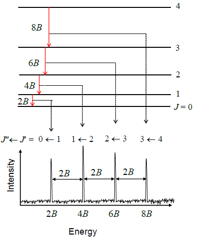
Figure \(\PageIndex{3}\) shows the rotational spectrum as a series of nearly equally spaced lines. The line positions \(\nu _J\), line spacings, and the maximum absorption coefficients ( \(\gamma _{max}\), the absorption coefficients associated with the specified line position) for each line in this spectrum are given here in Table \(\PageIndex{1}\).
|
|
|
|
|
|---|---|---|---|
| \(0 \rightarrow 1\) | 115,271.21 | 0 | 0.0082 |
| \(1 \rightarrow 2\) | 230,538.01 | 115,266.80 | 0.0533 |
| \(2 \rightarrow 3\) | 345,795.99 | 115,257.99 | 0.1278 |
| \(3 \rightarrow 4\) | 461,040.76 | 115,244.77 | 0.1878 |
| \(4 \rightarrow 5\) | 576,267.91 | 115,227.15 | 0.1983 |
| \(6 \rightarrow 6\) | 691,473.03 | 115,205.12 | 0.1618 |
| \(6 \rightarrow 7\) | 806,651.78 | 115,178.68 | 0.1064 |
| \(7 \rightarrow 8\) | 921,799.55 | 115,147.84 | 0.0576 |
| \(8 \rightarrow 9\) | 1,036,912.14 | 115,112.59 | 0.0262 |
| \(9 \rightarrow 10\) | 1,151,985.08 | 115,072.94 | 0.0103 |
Let’s try to reproduce Figure \(\PageIndex{3}\) from the data in Table \(\PageIndex{1}\) by using the quantum theory that we have developed so far. Equation \(\ref{5.9.8}\) predicts a pattern of exactly equally spaced lines. The lowest energy transition is between \(J_i = 0\) and \(J_f = 1\) so the first line in the spectrum appears at a frequency of \(2B\). The next transition is from \(J_i = 1\) to \(J_f = 2\) so the second line appears at \(4B\). The spacing of these two lines is \(2B\). In fact the spacing of all the lines is \(2B\), which is consistent with the experimental data in Table \(\PageIndex{1}\) showing that the lines are very nearly equally spaced. The difference between the first spacing and the last spacing is less than 0.2%.
Use Equation \(\ref{5.9.8}\) to prove that the spacing of any two lines in a rotational spectrum is \(2B\), i.e. derive:
\[\nu _{J_i + 1} - \nu _{J_i} = 2B \nonumber\]
- Answer
-
To prove the relationship, evaluate the LHS. First, define the terms:
\[ \upsilon_{J_{i}}=2B(J_{i}+1),\upsilon_{J_{i}+1}=2B((J_{i}+1)+1) \]
Substitute into the equation and evaluate:
\[2B((J_{i}+1)+1)-2B(J_{i}+1)=2B\]
\[2B(J_{i}+1)+2B-2B(J_{i}+1)=2B\]
\[2B=2B\]
LHS equals RHS.Therefore, the spacing between any two lines is equal to 2B.
The molecule \(NaH\) undergoes a rotational transition from \(J=0\) to \(J=1\) when it absorbs a photon of frequency \(2.94 \times 10^{11} \ Hz\). What is the equilibrium bond length of the molecule?
Solution
We use \(J=0\) in the formula for the transition frequency
Solving for \(R_e\) gives
The reduced mass is given by
\[\begin{align*}\mu &= \dfrac{m_{Na}m_H}{m_{Na}+m_H}=\dfrac{(22.989)(1.0078)}{22.989+1.0078}\\ &=0.9655\end{align*} \nonumber\]
which is in atomic mass units or relative units. To convert to kilograms, we need the conversion factor \(1 \ au = 1.66\times 10^{-27} \ kg\). Multiplying this by \(0.9655\) gives a reduced mass of \(1.603\times 10^{-27} \ kg\). Substituting in for \(R_e\) gives
\[\begin{align*}R_e &= \sqrt{\dfrac{(1.055 \times 10^{-34} \ J\cdot s)}{2\pi (1.603\times 10^{-27} \ kg)(2.94\times 10^{11} \ Hz)}}\\ &= 1.899\times 10^{-10} \ m=1.89 \ \stackrel{\circ}{A}\end{align*}\]
Use the frequency of the \(J = 0\) to \(J = 1\) transition observed for carbon monoxide to determine a bond length for \(^{12}C^{16}O\).
Centrifugal stretching of the bond as \(J\) increases causes the decrease in the spacing between the lines in an observed spectrum (Table \(\PageIndex{1}\)). This decrease shows that the molecule is not really a rigid rotor. As the rotational angular momentum increases with increasing \(J\), the bond stretches. This stretching increases the moment of inertia and decreases the rotational constant (Figure \(\PageIndex{5}\)).
The effect of centrifugal stretching is smallest at low \(J\) values, so a good estimate for \(B\) can be obtained from the \(J = 0\) to \(J = 1\) transition. From \(B\), a value for the bond length of the molecule can be obtained since the moment of inertia that appears in the definition of \(B\) (Equation \(\ref{5.9.9}\)) is the reduced mass times the bond length squared. When the centrifugal stretching is taken into account quantitatively, the development of which is beyond the scope of the discussion here, a very accurate and precise value for B can be obtained from the observed transition frequencies because of their high precision. Rotational transition frequencies are routinely reported to 8 and 9 significant figures.
As we have just seen, quantum theory successfully predicts the line spacing in a rotational spectrum. An additional feature of the spectrum is the line intensities. The lines in a rotational spectrum do not all have the same intensity, as can be seen in Figure \(\PageIndex{3}\) and Table \(\PageIndex{1}\). The maximum absorption coefficient for each line, \(\gamma _{max}\), is proportional to the magnitude of the transition moment, \(\mu _T\) which is given by Equation \(\ref{5.9.2}\), and to the population difference between the initial and final states, \(\Delta n\). Since \(\Delta n\) is the difference in the number of molecules present in the two states per unit volume, it is actually a difference in number density. This will be discussed in more detail in the following chapters
Contributors
David M. Hanson, Erica Harvey, Robert Sweeney, Theresa Julia Zielinski ("Quantum States of Atoms and Molecules")
Solution
\[ \Delta v=230538.01 M H z-115271.21 MHz=115266.8 M H z=1.153 \times 10^{11} H z=\frac{\hbar}{2 \pi \mu R_{e}}\]
The reduced mass is
\[\mu=\dfrac{m_{C} m_{O}}{m_{C}+m_{O}}=\frac{12.01 \times 16.00}{12.01+16.00}=6.86\, amu \]
Convert to kg
\[6.86 amu \, \frac{1.661 \times 10^{-27} k g}{12 m u}=1.139 \times 10^{-26} k g\]
\[\begin{aligned} R_{e}=\sqrt{\frac{\hbar}{2 \pi \mu \Delta v}}=& \sqrt{\frac{1.055 \times 10^{-34} J \cdot s}{2 \pi \cdot 1.139 \times 10^{-26} k g \cdot 1.153 \times 10^{11} H z}}=1.131 \times 10^{-10} \mathrm{m}=1.131 A \end{aligned}\)