
3.9: A Particle in a Three-Dimensional Box
- Page ID
- 210801
\( \newcommand{\vecs}[1]{\overset { \scriptstyle \rightharpoonup} {\mathbf{#1}} } \)
\( \newcommand{\vecd}[1]{\overset{-\!-\!\rightharpoonup}{\vphantom{a}\smash {#1}}} \)
\( \newcommand{\id}{\mathrm{id}}\) \( \newcommand{\Span}{\mathrm{span}}\)
( \newcommand{\kernel}{\mathrm{null}\,}\) \( \newcommand{\range}{\mathrm{range}\,}\)
\( \newcommand{\RealPart}{\mathrm{Re}}\) \( \newcommand{\ImaginaryPart}{\mathrm{Im}}\)
\( \newcommand{\Argument}{\mathrm{Arg}}\) \( \newcommand{\norm}[1]{\| #1 \|}\)
\( \newcommand{\inner}[2]{\langle #1, #2 \rangle}\)
\( \newcommand{\Span}{\mathrm{span}}\)
\( \newcommand{\id}{\mathrm{id}}\)
\( \newcommand{\Span}{\mathrm{span}}\)
\( \newcommand{\kernel}{\mathrm{null}\,}\)
\( \newcommand{\range}{\mathrm{range}\,}\)
\( \newcommand{\RealPart}{\mathrm{Re}}\)
\( \newcommand{\ImaginaryPart}{\mathrm{Im}}\)
\( \newcommand{\Argument}{\mathrm{Arg}}\)
\( \newcommand{\norm}[1]{\| #1 \|}\)
\( \newcommand{\inner}[2]{\langle #1, #2 \rangle}\)
\( \newcommand{\Span}{\mathrm{span}}\) \( \newcommand{\AA}{\unicode[.8,0]{x212B}}\)
\( \newcommand{\vectorA}[1]{\vec{#1}} % arrow\)
\( \newcommand{\vectorAt}[1]{\vec{\text{#1}}} % arrow\)
\( \newcommand{\vectorB}[1]{\overset { \scriptstyle \rightharpoonup} {\mathbf{#1}} } \)
\( \newcommand{\vectorC}[1]{\textbf{#1}} \)
\( \newcommand{\vectorD}[1]{\overrightarrow{#1}} \)
\( \newcommand{\vectorDt}[1]{\overrightarrow{\text{#1}}} \)
\( \newcommand{\vectE}[1]{\overset{-\!-\!\rightharpoonup}{\vphantom{a}\smash{\mathbf {#1}}}} \)
\( \newcommand{\vecs}[1]{\overset { \scriptstyle \rightharpoonup} {\mathbf{#1}} } \)
\( \newcommand{\vecd}[1]{\overset{-\!-\!\rightharpoonup}{\vphantom{a}\smash {#1}}} \)
\(\newcommand{\avec}{\mathbf a}\) \(\newcommand{\bvec}{\mathbf b}\) \(\newcommand{\cvec}{\mathbf c}\) \(\newcommand{\dvec}{\mathbf d}\) \(\newcommand{\dtil}{\widetilde{\mathbf d}}\) \(\newcommand{\evec}{\mathbf e}\) \(\newcommand{\fvec}{\mathbf f}\) \(\newcommand{\nvec}{\mathbf n}\) \(\newcommand{\pvec}{\mathbf p}\) \(\newcommand{\qvec}{\mathbf q}\) \(\newcommand{\svec}{\mathbf s}\) \(\newcommand{\tvec}{\mathbf t}\) \(\newcommand{\uvec}{\mathbf u}\) \(\newcommand{\vvec}{\mathbf v}\) \(\newcommand{\wvec}{\mathbf w}\) \(\newcommand{\xvec}{\mathbf x}\) \(\newcommand{\yvec}{\mathbf y}\) \(\newcommand{\zvec}{\mathbf z}\) \(\newcommand{\rvec}{\mathbf r}\) \(\newcommand{\mvec}{\mathbf m}\) \(\newcommand{\zerovec}{\mathbf 0}\) \(\newcommand{\onevec}{\mathbf 1}\) \(\newcommand{\real}{\mathbb R}\) \(\newcommand{\twovec}[2]{\left[\begin{array}{r}#1 \\ #2 \end{array}\right]}\) \(\newcommand{\ctwovec}[2]{\left[\begin{array}{c}#1 \\ #2 \end{array}\right]}\) \(\newcommand{\threevec}[3]{\left[\begin{array}{r}#1 \\ #2 \\ #3 \end{array}\right]}\) \(\newcommand{\cthreevec}[3]{\left[\begin{array}{c}#1 \\ #2 \\ #3 \end{array}\right]}\) \(\newcommand{\fourvec}[4]{\left[\begin{array}{r}#1 \\ #2 \\ #3 \\ #4 \end{array}\right]}\) \(\newcommand{\cfourvec}[4]{\left[\begin{array}{c}#1 \\ #2 \\ #3 \\ #4 \end{array}\right]}\) \(\newcommand{\fivevec}[5]{\left[\begin{array}{r}#1 \\ #2 \\ #3 \\ #4 \\ #5 \\ \end{array}\right]}\) \(\newcommand{\cfivevec}[5]{\left[\begin{array}{c}#1 \\ #2 \\ #3 \\ #4 \\ #5 \\ \end{array}\right]}\) \(\newcommand{\mattwo}[4]{\left[\begin{array}{rr}#1 \amp #2 \\ #3 \amp #4 \\ \end{array}\right]}\) \(\newcommand{\laspan}[1]{\text{Span}\{#1\}}\) \(\newcommand{\bcal}{\cal B}\) \(\newcommand{\ccal}{\cal C}\) \(\newcommand{\scal}{\cal S}\) \(\newcommand{\wcal}{\cal W}\) \(\newcommand{\ecal}{\cal E}\) \(\newcommand{\coords}[2]{\left\{#1\right\}_{#2}}\) \(\newcommand{\gray}[1]{\color{gray}{#1}}\) \(\newcommand{\lgray}[1]{\color{lightgray}{#1}}\) \(\newcommand{\rank}{\operatorname{rank}}\) \(\newcommand{\row}{\text{Row}}\) \(\newcommand{\col}{\text{Col}}\) \(\renewcommand{\row}{\text{Row}}\) \(\newcommand{\nul}{\text{Nul}}\) \(\newcommand{\var}{\text{Var}}\) \(\newcommand{\corr}{\text{corr}}\) \(\newcommand{\len}[1]{\left|#1\right|}\) \(\newcommand{\bbar}{\overline{\bvec}}\) \(\newcommand{\bhat}{\widehat{\bvec}}\) \(\newcommand{\bperp}{\bvec^\perp}\) \(\newcommand{\xhat}{\widehat{\xvec}}\) \(\newcommand{\vhat}{\widehat{\vvec}}\) \(\newcommand{\uhat}{\widehat{\uvec}}\) \(\newcommand{\what}{\widehat{\wvec}}\) \(\newcommand{\Sighat}{\widehat{\Sigma}}\) \(\newcommand{\lt}{<}\) \(\newcommand{\gt}{>}\) \(\newcommand{\amp}{&}\) \(\definecolor{fillinmathshade}{gray}{0.9}\)- To see the particle in 1-D box can easily extrapolate to boxes of higher dimensions.
- Introduction to nodal surfaces (e.g., nodal planes)
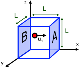
The quantum particle in the 1D box problem can be expanded to consider a particle within a higher dimensions as demonstrated elsewhere for a quantum particle in a 2D box. Here we continue the expansion into a particle trapped in a 3D box with three lengths \(L_x\), \(L_y\), and \(L_z\). As with the other systems, there is NO FORCE (i.e., no potential) acting on the particles inside the box (Figure \(\PageIndex{1}\)).
The potential for the particle inside the box
\[V(\vec{r}) = 0\]
- \(0 \leq x \leq L_x\)
- \(0 \leq y \leq L_y\)
- \(0 \leq z \leq L_z\)
- \(L_x < x < 0\)
- \(L_y < y < 0\)
- \(L_z < z < 0\)
\(\vec{r}\) is the vector with all three components along the three axes of the 3-D box: \(\vec{r} = L_x\hat{x} + L_y\hat{y} + L_z\hat{z}\). When the potential energy is infinite, then the wavefunction equals zero. When the potential energy is zero, then the wavefunction obeys the Time-Independent Schrödinger Equation
\[-\dfrac{\hbar^{2}}{2m}\nabla^{2}\psi(r) + V(r)\psi(r) = E\psi(r) \label{3.9.1}\]
Since we are dealing with a 3-dimensional figure, we need to add the 3 different axes into the Schrondinger equation:
\[-\dfrac{\hbar^{2}}{2m}\left(\dfrac{d^{2}\psi(r)}{dx^{2}} + \dfrac{d^{2}\psi(r)}{dy^{2}} + \dfrac{d^{2}\psi(r)}{dz^{2}}\right) = E\psi(r) \label{3.9.2}\]
The easiest way in solving this partial differential equation is by having the wavefunction equal to a product of individual function for each independent variable (e.g., the Separation of Variables technique):
\[\psi{(x,y,z)} = X(x)Y(y)Z(z) \label{3.9.3}\]
Now each function has its own variable:
- \(X(x)\) is a function for variable \(x\) only
- \(Y(y)\) function of variable \(y\) only
- \(Z(z)\) function of variable \(z\) only
Now substitute Equation \(\ref{3.9.3}\) into Equation \(\ref{3.9.2}\) and divide it by the product: \(xyz\):
\[\dfrac{d^{2}\psi}{dx^{2}} = YZ\dfrac{d^{2}X}{dx^{2}} \Rightarrow \dfrac{1}{X}\dfrac{d^{2}X}{dx^{2}}\]
\[\dfrac{d^{2}\psi}{dy^{2}} = XZ\dfrac{d^{2}Y}{dy^{2}} \Rightarrow \dfrac{1}{Y}\dfrac{d^{2}Y}{dy^{2}}\]
\[\dfrac{d^{2}\psi}{dz^{2}} = XY\dfrac{d^{2}Z}{dz^{2}} \Rightarrow \dfrac{1}{Z}\dfrac{d^{2}Z}{dz^{2}}\]
\[\left(-\dfrac{\hbar^{2}}{2mX} \dfrac{d^{2}X}{dx^{2}}\right) + \left(-\dfrac{\hbar^{2}}{2mY} \dfrac{d^{2}Y}{dy^{2}}\right) + \left(-\dfrac{\hbar^{2}}{2mZ} \dfrac{d^{2}Z}{dz^{2}}\right) = E \label{3.9.4}\]
\(E\) is an energy constant, and is the sum of x, y, and z. For this to work, each term must equal its own constant. For example,
\[\dfrac{d^{2}X}{dx^{2}} + \dfrac{2m}{\hbar^{2}} \varepsilon_{x}X = 0\]
Now separate each term in Equation \(\ref{3.9.4}\) to equal zero:
\(\dfrac{d^{2}X}{dx^{2}} + \dfrac{2m}{\hbar^{2}} \varepsilon_{x}X = 0 \label{3.9.5a}\)
\(\dfrac{d^{2}Y}{dy^{2}} + \dfrac{2m}{\hbar^{2}} \varepsilon_{y}Y = 0 \label{3.9.5b}\)
\(\dfrac{d^{2}Z}{dz^{2}} + \dfrac{2m}{\hbar^{2}} \varepsilon_{z}Z = 0 \label{3.9.5c}\)
Now we can add all the energies together to get the total energy:
\[\varepsilon_{x}+ \varepsilon_{y} + \varepsilon_{z} = E \label{3.9.6}\]
Do these equations look familiar? They should because we have now reduced the 3D box into three particle in a 1D box problems!
\[\dfrac{d^{2}X}{dx^{2}} + \dfrac{2m}{\hbar^{2}} E_{x}X = 0 \approx \dfrac{d^{2}\psi}{dx^{2}} = -\dfrac{4\pi^{2}}{\lambda^{2}}\psi \label{3.9.7}\]
Now the equations are very similar to a 1-D box and the boundary conditions are identical, i.e.,
\[n = 1, 2,..\infty\]
Use the normalization wavefunction equation for each variable:
\[\psi(x) =
\begin{cases}
\sqrt{\dfrac{2}{L_x}}\sin{\dfrac{n \pi x}{L_x}} & \mbox{if } 0 \leq x \leq L \\
0 & \mbox{if } {L < x < 0}
\end{cases}\]
Normalization wavefunction equation for each variable
\[X(x) = \sqrt{\dfrac{2}{L_x}} \sin \left( \dfrac{n_{x}\pi x}{L_x} \right) \label{3.9.8a}\]
\[Y(y) = \sqrt{\dfrac{2}{L_y}} \sin \left(\dfrac{n_{y}\pi y}{L_y} \right) \label{3.9.8b}\]
\[Z(z) = \sqrt{\dfrac{2}{L_z}} \sin \left( \dfrac{n_{z}\pi z}{L_z} \right) \label{3.9.8c}\]
The limits of the three quantum numbers
- \(n_{x} = 1, 2, 3, ...\infty\)
- \(n_{y} = 1, 2, 3, ...\infty\)
- \(n_{z} = 1, 2, 3, ...\infty\)
For each constant use the de Broglie Energy equation:
\[\varepsilon_{x} = \dfrac{n_{x}^{2}h^{2}}{8mL_x^{2}} \label{3.9.9}\]
with \(n_{x} = 1...\infty\)
Do the same for variables \(n_y\) and \(n_z\). Combine Equation \(\ref{3.9.3}\) with Equations \(\ref{3.9.8a}\)-\(\ref{3.9.8c}\) to find the wavefunctions inside a 3D box.
\[\psi(r) = \sqrt{\dfrac{8}{V}}\sin \left( \dfrac{n_{x} \pi x}{L_x} \right) \sin \left(\dfrac{n_{y} \pi y}{L_y}\right) \sin \left(\dfrac{ n_{z} \pi z}{L_z} \right) \label{3D wave}\]
with
\[V = \underbrace{L_x \times L_y \times L_z}_{\text{volume of box}}\]
To find the Total Energy, add Equation \(\ref{3.9.9}\) and Equation \(\ref{3.9.6}\).
\[E_{n_x,n_y,n_z} = \dfrac{h^{2}}{8m}\left(\dfrac{n_{x}^{2}}{L_x^{2}} + \dfrac{n_{y}^{2}}{L_y^{2}} + \dfrac{n_{z}^{2}}{L_z^{2}}\right) \label{3.9.10}\]
Notice the similarity between the energies a particle in a 3D box (Equation \(\ref{3.9.10}\)) and a 1D box.
Degeneracy in a 3D Cube
The energy of the particle in a 3-D cube (i.e., \(a=L\), \(b=L\), and \(c= L\)) in the ground state is given by Equation \(\ref{3.9.10}\) with \(n_x=1\), \(n_y=1\), and \(n_z=1\). This energy (\(E_{1,1,1}\)) is hence
\[E_{1,1,1} = \dfrac{3 h^{2}}{8mL^2}\]
The ground state has only one wavefunction and no other state has this specific energy; the ground state and the energy level are said to be non-degenerate. However, in the 3-D cubical box potential the energy of a state depends upon the sum of the squares of the quantum numbers (Equation \ref{3D wave}). The particle having a particular value of energy in the excited state MAY has several different stationary states or wavefunctions. If so, these states and energy eigenvalues are said to be degenerate.
For the first excited state, three combinations of the quantum numbers \((n_x,\, n_y, \, n_z )\) are \((2,\,1,\,1),\, (1,2,1),\, (1,1,2)\). The sum of squares of the quantum numbers in each combination is same (equal to 6). Each wavefunction has same energy:
\[E_{2,1,1} =E_{1,2,1} = E_{1,1,2} = \dfrac{6 h^{2}}{8mL^2}\]
Corresponding to these combinations three different wavefunctions and three different states are possible. Hence, the first excited state is said to be three-fold or triply degenerate. The number of independent wavefunctions for the stationary states of an energy level is called as the degree of degeneracy of the energy level. The value of energy levels with the corresponding combinations and sum of squares of the quantum numbers
\[n^2 \,= \, n_x^2+n_y^2+n_z^2\]
as well as the degree of degeneracy are depicted in Table \(\PageIndex{1}\).
| \(n_x^2+n_y^2+n_z^2\) | Combinations of Degeneracy (\(n_x\), \(n_y\), \(n_z\)) |
Total Energy (\(E_{n_x,n_y,n_z}\)) |
Degree of Degeneracy | |||||
|---|---|---|---|---|---|---|---|---|
| 3 | (1,1,1) | \(\dfrac{3 h^{2}}{8mL^2}\) | 1 | |||||
| 6 | (2,1,1) | (1,2,1) | (1,1,2) | \(\dfrac{6 h^{2}}{8mL^2}\) | 3 | |||
| 9 | (2,2,1) | (1,2,2) | (2,1,2) | \(\dfrac{9 h^{2}}{8mL^2}\) | 3 | |||
| 11 | (3,1,1) | (1,3,1) | (1,1,3) | \(\dfrac{11 h^{2}}{8mL^2}\) | 3 | |||
| 12 | (2,2,2) | \(\dfrac{12 h^{2}}{8mL^2}\) | 1 | |||||
| 14 | (3,2,1) | (3,1,2) | (2,3,1) | (2,1,3) | (1,3,2) | (1,2,3) | \(\dfrac{14 h^{2}}{8mL^2}\) | 6 |
| 17 | (2,2,3) | (3,2,2) | (2,3,2) | \(\dfrac{17 h^{2}}{8mL^2}\) | 3 | |||
| 18 | (1,1,4) | (1,4,1) | (4,1,1) | \(\dfrac{18 h^{2}}{8mL^2}\) | 3 | |||
| 19 | (1,3,3) | (3,1,3) | (3,3,1) | \(\dfrac{19 h^{2}}{8mL^2}\) | 3 | |||
| 21 | (1,2,4) | (1,4,2) | (2,1,4) | (2,4,1) | (4,1,2) | (4,2,1) | \(\dfrac{21 h^{2}}{8mL^2}\) | 6 |
When is there degeneracy in a 3-D box when none of the sides are of equal length (i.e., \(L_x \neq L_y \neq L_z\))?
Solution
From simple inspection of Equation \ref{3.9.10} or Table \(\PageIndex{1}\), it is clear that degeneracy originates from different combinations of \(n_x^2/L_x^2\), \(n_y^2/L_y^2\) and \(n_z^2/L_z^2\) that give the same value. These will occur at common multiples of at least two of these quantities (the Least Common Multiple is one example). For example
if
\[\dfrac{n_x^2}{L_x^2} = \dfrac{n_y^2}{L_y^2} \nonumber\]
there will be a degeneracy. Also degeneracies will exist if
\[\dfrac{n_y^2}{L_y^2} = \dfrac{n_z^2}{L_z^2} \nonumber\]
or if
\[\dfrac{n_x^2}{L_x^2} = \dfrac{n_z^2}{L_z^2} \nonumber\]
and especially if
\[\dfrac{n_x^2}{L_x^2} = \dfrac{n_y^2}{L_y^2} = \dfrac{n_z^2}{L_z^2} \nonumber.\]
There are two general kinds of degeneracies in quantum mechanics: degeneracies due to a symmetry (i.e., \(L_x=L_y\)) and accidental degeneracies like those above.
The 6th energy level of a particle in a 3D Cube box is 6-fold degenerate.
- What is the energy of the 7th energy level?
- What is the degeneracy of the 7th energy level?
- Answer a
-
\(\dfrac{17 h^{2}}{8mL^2}\)
- Answer b
-
three-fold (i.e., there are three wavefunctions that share the same energy.
References
- Atkins, Peter. Physical Chemistry 5th Ed. USA. 1994.
- Fitts, Donald. Principles of Quantum Mechanics. United Kingdom, Cambridge. University Press. 1999
- McQuarrie. Donald. Physical Chemistry A Molecular Approach. Sausalito, CA. University Science Books. 1997.
- Riggs. N. V. Quantum Chemistry. Toronto, Ontario. The Macmillan Company. 1969
- C. A. Hollingsworth, Accidental Degeneracies of the Particle in a Box, J. Chem. Educ., 1990, 67 (12), p 999