8.11: Oscillating Reactions

It should be clear by now that chemical kinetics is governed by the mathematics of systems of differential equations. Thus far, we have only looked at reaction systems that give rise to purely linear differential equations, however, in many instances the rate equations are nonlinear. When the differential equations are nonlinear, the behavior is considerably more complex. In particular, nonlinear equations can lead to oscillatory solutions and can also exhibit the phenomenon of chaos. Chaotic systems are systems that are highly sensitive to small changes in the parameters of the equations or in the initial conditions. Basically, this means that the behavior of a chaotic system can be unpredictable, since such small changes can occur in the form of small errors in determining the parameters (rounding to the nearest tenth or hundredth) or in specifying the initial conditions, and these small changes can cause the system to evolve in time in a very different way.

The Iodine Clock Reaction

The iodine clock reaction is a popular chemistry experiment in which one can visualize how different rate constants in consecutive reactions affect the concentration of species during the reaction. Iodine anions ($I^-$) are colorless. When $I^-$ is reacted with hydrogen peroxide and protons, triiodide is formed, which has a dark blue color. Consider the following series of irreversible reactions:

$$H_2 O_2 + 3 \: I^- + 2 \: H^+ \overset{k_1}{\longrightarrow} I_3^- + 2 \: H_2O$$

$$I_3^- + 2 \: S_2 O_3^{2-} \overset{k_2}{\longrightarrow} 3 \: I^- + S_4 O_6^{2-}$$

The rate laws for this system are

$$\begin{align} \dfrac{ d \left[ I_3^- \right]}{dt} &= k_1 \left[ I^- \right]^3 - k_2 \left[ I_3^- \right] \left[ S_2 O_3^{2-} \right]^2 \\ \dfrac{d \left[ I^- \right]}{dt} &= -k_1 \left[ I^- \right]^3 + 3k_2 \left[ I_3^- \right] \left[ S_2 O_3^{2-} \right]^2 \\ \dfrac{d \left[ S_2 O_3^{2-} \right]}{dt} &= -k_2 \left[ I_3^- \right] \left[ S_2 O_3^{2-} \right]^2 \end{align} \label{Eq2}$$

In order to make the equations look a little simpler, let us introduce the variables:

$$x = \left[ I^- \right], \: \: \: \: \: \: \: y = \left[ I_3^- \right], \: \: \: \: \: \: \: z = \left[ S_2 O_3^{2-} \right] \label{Eq3}$$

In terms of these, the rate equations are

$$\begin{align} \dfrac{dx}{dt} &= -k_1 x^3 + 3 k_2 yz^2 \\ \dfrac{dy}{dt} &= k_1 x^3 - k_2 yz^2 \\ \dfrac{dz}{dt} &= -k_2 yz^2 \end{align} \label{Eq4}$$

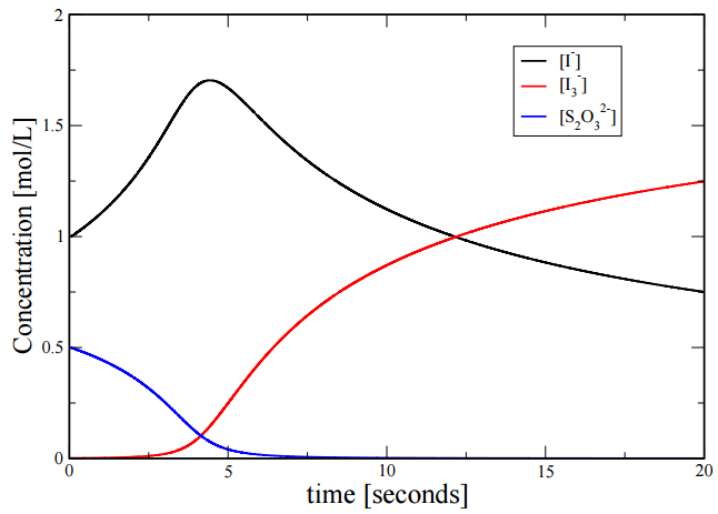
If we solve these numerically, we find the following time dependence of the three concentrations: This is a clear example of nonlinearity. Note how the concentration of $I_3^-$ remains close to $0$ for a period of time and then suddenly starts to increase. In a sense, think of the “straw that broke the camel’s back”. As we pile straws on the back of the camel, the camel remains upright until that last straw, which suddenly breaks the back of the camel, and the camel suddenly falls to the ground. This is also an illustration of nonlinearity.

Video $\PageIndex{1}$: Famous iodine clock reaction: oxidation of potassium iodide by hydrogen peroxide (https://www.youtube.com/watch?v=_qhYDuJt8fI).

Despite the complexity of the rate equations, we can still analyze the approximately and predict the behavior seen in Figure $\PageIndex{1}$. In this reaction mechanism, $k_2 \gg k_1$. Given the rate law for $I_3^-$,

$$\dfrac{d \left[ I_3^- \right]}{dt} = k_1 \left[ I^- \right]^3 - k_2 \left[ I_3^- \right] \left[ S_2 O_3^{2-} \right]^2 \label{Eq5}$$

if we use the steady-state approximation, we can set the $\dfrac{d \left[ I_3^- \right]}{dt}$ equal to $0$, yielding

$$\left[ I_3^- \right] = \dfrac{k_1}{k_2} \dfrac{\left[ I^- \right]^3}{\left[ S_2 O_3^{2-} \right]^2} \label{Eq6}$$

Since $k_2 \gg k_1$, the concentration of $\left[ I_3^- \right]$ is approximately $0$ as long as there are $S_2 O_3^{2-}$ ions present. As soon as all of the $S_2 O_3^{2-}$ is consumed, the concentration of $I_3^-$ can build up in the solution, changing the solution to a dark blue color. Figure $\PageIndex{1}$ displays the concentration profiles for $I^-$, $I_3^-$, and $S_3 O_3^{2-}$. As can be seen from the figure, the concentration of $I_3^-$ (red line) remains at approximately $0 \: \text{mol/L}$ until all of the $S_2 O_3^{2-}$ (blue line) has been depleted.

Figure $\PageIndex{1}$: Concentrations as functions of time of the three species in the iodine clock reaction.

Oscillating Reactions

In all of the examples we have seen thus far, the concentration of intermediate species displays a single maximum during the course of the reaction. There is another class of reactions called oscillating reactions in which the concentration of intermediate species oscillates with time. Consider the following series of reactions

$$\text{A} + \text{Y} \overset{k_1}{\longrightarrow} \text{X}$$

$$\text{X} + \text{Y} \overset{k_2}{\longrightarrow} \text{P}$$

$$\text{B} + \text{X} \overset{k_3}{\longrightarrow} 2 \: \text{X} + \text{Z}$$

$$2 \: \text{X} \overset{k_4}{\longrightarrow} \text{Q}$$

$$\text{Z} \overset{k_5}{\longrightarrow} \text{Y}$$

In the above reaction mechanism, $\text{A}$ and $\text{B}$ are reactants; $\text{X}$, $\text{Y}$, and $\text{Z}$ are intermediates; and $\text{P}$ and $\text{Q}$ are products. The third reaction in which $\text{B}$ and $\text{X}$ react to form $\text{X}$ and $\text{Z}$ is known as an ”autocatalytic reaction” in which at least one of the reactants is also a product. Such reactions are a key feature of oscillating reactions, as will be discussed below.

Video $\PageIndex{2}$: The famous Belousov Zhabotinsky chemical reaction in a petri dish. The action is speeded up 8 x from real life. Pacemaker nucleation sites emit circular waves. Breaking the wavefront with a wire triggers pairs of spiral defects which emit more closely spaced waves which eventually fill the container.

Let us assume that the concentrations of $\text{A}$ and $\text{B}$ are large, such that we can approximate them to be constant with time. The rate equation for species $\text{X}$ can be written as

$$\dfrac{d \left[ \text{X} \right]}{dt} = k_1 \left[ \text{A} \right] \left[ \text{Y} \right] - k_2 \left[ \text{X} \right] \left[ \text{Y} \right] + k_3 \left[ \text{B} \right] \left[ \text{X} \right] - 2k_4 \left[ \text{X} \right]^2 \label{Eq7}$$

Using the steady-state approximation, we can set $d \text{X}/dt = 0$ and rewrite Equation $\ref{Eq7}$ as

$$\left( -2 k_4 \right) \left[ \text{X} \right]^2 + \left( k_2 \left[ \text{Y} \right] - k_3 \left[ \text{B} \right] \right) \left[ \text{X} \right] + k_1 \left[ \text{A} \right] \left[ \text{Y} \right] = 0 \label{Eq8}$$

We can then use the quadratic formula to solve for $\text{X}$:

$$\left[ \text{X} \right] = -\dfrac{ \left( k_2 \left[ \text{Y} \right] - k_3 \left[ \text{B} \right] \right) \pm \sqrt{\left( k_2 \left[ \text{Y} \right] - k_3 \left[ \text{B} \right] \right)^2 - 4 \left( -2k_4 \right) \left( k_1 \left[ \text{A} \right] \left[ \text{Y} \right] \right)}}{2 \left( -2k_4 \right)} \label{Eq9}$$

Thus, there are two solutions for the concentration of $\text{X}$ accessible to the reaction system. To examine solutions for $\left[ \text{X} \right]$, let us first assume that $\left[ \text{Y} \right]$ is large. Under these conditions, the first two reactions in the reaction mechanism largely determine the concentration of $\left[ \text{X} \right]$. We can thus approximate Equation $\ref{Eq7}$ as

$$0 \approx k_1 \left[ \text{A} \right] \left[ \text{Y} \right] - k_2 \left[ \text{X} \right] \left[ \text{Y} \right] \label{Eq10}$$

Solving for $\left[ \text{X} \right]$ yields

$$\left[ \text{X} \right] \approx \dfrac{k_1 \left[ \text{A} \right]}{k_2} \label{Eq11}$$

As the reaction continues, species $\text{Y}$ is depleted and the assumption that $\left[ \text{Y} \right]$ is large becomes invalid. Instead the $3^{rd}$ and $4^{th}$ steps of the reaction mechanism determine the concentration of $\text{X}$. In this limit, we can approximate Equation $\ref{Eq7}$ as

$$0 \approx k_3 \left[ \text{B} \right] \left[ \text{X} \right] - 2 k_4 \left[ \text{X} \right]^2 \label{Eq12}$$

Solving for $\left[ \text{X} \right]$ yields

$$\left[ \text{X} \right] \approx \dfrac{k_3 \left[ \text{B} \right]}{2k_4} \label{Eq13}$$

In the second mechanism, the autocatalytic reaction step leads to an increase in the concentration of $\text{X}$ and $\text{Z}$, which in turn leads to an increase in the concentration of $\text{Y}$. The feedback loop between the production of species $\text{X}$ and $\text{Y}$ leads to oscillatory behavior in the system. This reaction mechanism is known as the Belousov-Zhabotinksii reaction first discovered in the 1950s.

• The autocatalytic reaction of $\text{X}$ in which $\text{X}$ reacts with $\text{B}$ to form more $\text{X}$ in reaction $3$
• The regeneration of species $\text{Y}$ in reaction $5$
• The competition between reaction $2$ and $3$ for the consumption of $\text{X}$ and the involvement of $\text{Y}$ in reaction $2$

The actual Belousov-Zhabotinskii reaction is complex, involving many individual steps, and involves the oscillation between the concentration of $HBrO_2$ and $Br^-$. The reaction equations are

$$\begin{align} BrO_3^- + Br^- + 2 \: H^+ &\longrightarrow HBrO_2 + HOBr \\ HBrO_2 + Br^- + H^+ &\longrightarrow 2 \: HOBr \\ HOBr + Br^- + H^+ &\longrightarrow Br_2 + H_2 O \\ 2 \: HBrO_2 &\longrightarrow BrO_3^- + HOBr + H^+ \\ BrO_3^- + HBrO_2 + H^+ &\longrightarrow 2 \: BrO_2^. + H_2 O \\ BrO_2^. + Ce^{3+} + H^+ &\longrightarrow HBrO_2 + Ce^{4+} \\ BrO_2^. + Ce^{4+} + H_2 O &\longrightarrow BrO_3^- + Ce^{3+} + 2 \: H^+ \end{align} \label{Eq14}$$

The essential steps in this mechanism can be reduced to the following set of reactions. Note that we leave this unbalanced and only include the species whose concentrations as functions of time we seek.

$$\begin{align} BrO_3^- + Br^- &\overset{k_1}{\longrightarrow} HBrO_2 + HOBr \\ HBrO_2 + Br^- &\overset{k_2}{\longrightarrow} 2 \: HOBr \\ BrO_3^- + HBrO_2 &\overset{k_3}{\longrightarrow} 2 \: HBrO_2 + 2 \: Ce^{4+} \\ 2 \: HBrO_2 &\overset{k_4}{\longrightarrow} BrO_3^- + HOBr \\ Ce^{4+} &\overset{k_5}{\longrightarrow} fBr^- \end{align} \label{Eq15}$$

Setting the variables as follows:

$$x = \left[ HBrO_2 \right], \: \: \: \: \: \: \: y = \left[ Br^- \right], \: \: \: \: \: \: \: z = \left[ Ce^{4+} \right] \label{Eq16}$$

We make the approximation that $\left[ BrO_3^- \right]$ to be a constant $a$. In this case, the rate equations become

$$\begin{align} \dfrac{dx}{dt} &= k_1 ay - k_2 xy + k_3 ax - k_4 x^2 \\ \dfrac{dy}{dt} &= -k_1 ay - k_2 xy + f k_5 z \\ \dfrac{dz}{dt} &= 2k_3 ax - k_5 z \end{align} \label{Eq17}$$

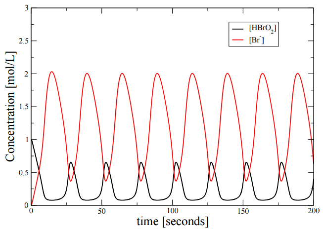
Solving these equations numerically, we obtain the trajectory of two of the species show in the Figure $\PageIndex{2}$.

Figure $\PageIndex{2}$: Oscillating pattern of the concentrations in the Belousov-Zhabotinskii reaction.

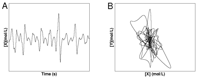
On the other hand, we can drive this system to become chaotic by changing the parameters a little. When this is done, we find the follow plot of the concentration of $x$:

Figure $\PageIndex{3}$: Chaotic behavior in the Belousov-Zhabotinskii reaction.

Contributors

• Mark Tuckerman (New York University)