8.10: Fast Reactions in Solution

The traditional experimental methods described above all assume the possibility of following the reaction after its components have combined into a homogeneous mixture of known concentrations. But what can be done if the time required to complete the mixing process is comparable to or greater than the time needed for the reaction to run to completion?

Flow methods

Flow instruments are a rapid mixing devices used to study the chemical kinetics of fast reactions in solution. There are different flavors that can be implement depending on the nature of the reaction as discussed below.

Continuous Flow Approach

For reactions that take place in milliseconds, the standard approach since the 1950s has been to employ a flow technique of some kind. An early example was used to study fast gas-phase reactions in which one of the reactants is a free radical such as OH that can be produced by an intense microwave discharge acting on a suitable source gas mixture. This gas, along with the other reactant being investigated, is made to flow through a narrow tube at a known velocity.

Figure \(\PageIndex{1}\): A continuous flow fast kinetic system.

If the distance between the point at which the reaction is initiated and the product detector is known, then the time interval can be found from the flow rate. By varying this distance, the time required to obtain the maximum yield can then be determined. Although this method is very simple in principle, it can be complicated in practice.

Stopped Flow Approach

Owing to the rather large volumes required, continuous flow method is more practical for the study of gas-phase reactions than for solutions, for which the stopped-flow method described below is generally preferred. These are by far the most common means of studying fast solution-phase reactions over time intervals of down to a fraction of a millisecond. The use of reasonably simple devices is now practical even in student laboratory experiments. These techniques make it possible to follow not only changes in the concentrations of reactants and products, but also the buildup and decay of reaction intermediates.

Figure \(\PageIndex{2}\): A stop flow fast kinetic system.

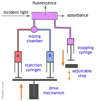
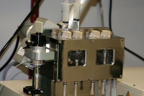
The basic stopped-flow apparatus consists of two or more coupled syringes that rapidly inject the reactants into a small mixing chamber and then through an observation cell that can be coupled to instruments that measure absorption, fluorescence, light scattering, or other optical or electrical properties of the solution. As the solution flows through the cell, it empties into a stopping syringe that, when filled, strikes a backstop that abruptly stops the flow. The volume that the stopping syringe can accept is adjusted so that the mixture in the cell has just become uniform and has reached a steady state; at this point, recording of the cell measurement begins and its change is followed.

Figure \(\PageIndex{3}\): Stop-flow equipment at a biochemistry research laboratory for measuring rapid reactions and properties such as enzyme kinetics. Image used with permission from Wladimir Labeikovsky.

Quenched Flow Approach

In a quenched-flow instrument, the reaction is stopped after a certain amount of time has passed after mixing. The stopping of the reaction is called quenching and it can be achieved by various means, for example by mixing with another solution, which stops the reaction (chemical quenching), quickly lowering the temperature (freeze quenching) or even by exposing the sample to light of a certain wavelength (optical quenching).

Of course, there are many reactions that cannot be followed by changes in light absorption or other physical properties that are conveniently monitored. In such cases, it is often practical to quench (stop) the reaction after a desired interval by adding an appropriate quenching agent. For example, an enzyme-catalyzed reaction can be stopped by adding an acid, base, or salt solution that denatures (destroys the activity of) the protein enzyme. Once the reaction has been stopped, the mixture is withdrawn and analyzed in an appropriate manner.

Figure \(\PageIndex{4}\): A quench flow fast kinetic system.

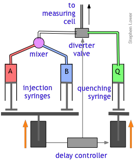
The quenched-flow technique works something like the stopped-flow method described above, with a slightly altered plumbing arrangement. The reactants A and B are mixed and fed directly through the diverter valve to the measuring cell, which is not shown in this diagram. After a set interval that can vary from a few milliseconds to 200 sec or more, the controller activates the quenching syringe and diverter valve, flooding the cell with the quenching solution.

Relaxation Methods

To investigate reactions that are complete in less than a millisecond, one can start with a pre-mixed sample in which one of active reactants is generated in situ. Alternatively, a rapid change in pressure or temperature can alter the composition of a reaction that has already achieved equilibrium.

Flash Photolysis

Many reactions are known which do not take place without light of wavelength sufficiently short to supply the activation energy needed to break a bond, often leading to the creation of a highly reactive radical. A good example is the combination of gaseous Cl₂ with H₂, which proceeds explosively when the system is illuminated with visible light. In flash photolysis, a short pulse of light is used to initiate a reaction whose progress can be observed by optical or other means.

Photolysis refers to the use of light to decompose a molecule into simpler units, often ions or free radicals. In contrast to thermolysis (decomposition induced by high temperature), photolysis is able to inject energy into a molecule almost instantaneously and can be much "cleaner," meaning that there are fewer side reactions that often lead to complex mixtures of products. Photolysis can also be highly specific; the wavelength of the light that triggers the reaction can often be adjusted to activate one particular kind of molecule without affecting others that might be present.

Norrish and Porter

All this had been known for a very long time, but until the mid-1940's there was no practical way of studying the kinetics of the reactions involving the highly reactive species produced by photolysis. In 1945, Ronald Norrish of Cambridge University and his graduate student George Porter conceived the idea of using a short-duration flash lamp to generate gas-phase CH₂ radicals, and then following the progress of the reaction of these radicals with other species by means of absorption spectroscopy.

Figure \(\PageIndex{5}\): Basic principle of a flash-photolysis relaxation experiment where an excitation pulse purturbed a system at equilibrium and the subsequent dynamics are resolved in time.

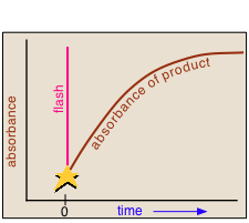
In a flash photolysis experiment, recording of the absorbance of the sample cell contents is timed to follow the flash by an interval that can be varied in order to capture the effects produced by the product or intermediate as it is formed or decays. Norrish and Porter shared the 1967 Nobel Prize in Chemistry for this work.

Figure \(\PageIndex{6}\): A flash-photolysis relaxation experiment

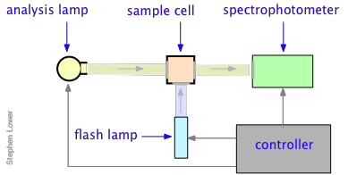
Many reactions, especially those that take place in solution, occur too rapidly to follow by flow techniques, and can therefore only be observed when they are already at equilibrium. The classical examples of such reactions are two of the fastest ones ever observed, the dissociation of water

\[ 2 H_2O \rightarrow H_3O^+ + OH^- \]

and the formation of the triiodide ion in aqueous solution

\[ I^– + I_2 \rightarrow I_3^–\]

Reactions of these kinds could not be studied until the mid-1950s when techniques were developed to shift the equilibrium by imposing an abrupt physical change on the system.

Temperature Jumps

The rate constants of reversible reactions can be measured using a relaxation method. In this method, the concentrations of reactants and products are allowed to achieve equilibrium at a specific temperature. Once equilibrium has been achieved, the temperature is rapidly changed, and then the time needed to achieve the new equilibrium concentrations of reactants and products is measured. For example, if the reaction

\[\text{A} \overset{k_1}{\underset{k_{-1}}{\rightleftharpoons}} \text{B} \label{relax}\]

is endothermic, then according to the Le Chatelier principle, subjecting the system to a rapid jump in temperature will shift the equilibrium state to one in which the product B has a higher concentration. The composition of the system will than begin to shift toward the new equilibrium composition at a rate determined by the kinetics of the process.

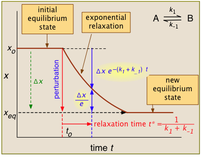
For the general case illustrated here, the quantity "x" being plotted is a measurable quantity such as light absorption or electrical conductivity that varies linearly with the composition of the system. In a first-order process, x will vary with time according to

\[ x_t = x_o e^{-kt} \]

After the abrupt perturbation at time t_o, the relaxation time t* is defined as the half-time for the return to equilibrium — that is, as the time required for \(x_o\) to decrease by \(Δx/e = Δx/2.718\). The derivation of t* and the relations highlighted in yellow can be found in most standard kinetics textbooks. Temperature jumps are likely most commonly used.

The rate law for the reversible reaction in Equation \(\ref{relax}\) can be written as

\[\dfrac{d \left[ \text{B} \right]}{dt} = k_1 \left[ \text{A} \right] - k_{-1} \left[ \text{B} \right] \label{19.33}\]

Consider a system comprising \(\text{A}\) and \(\text{B}\) that is allowed to achieve equilibrium concentrations at a temperature, \(T_1\). After equilibrium is achieved, the temperature of the system is instantaneously lowered to \(T_2\) and the system is allowed to achieve new equilibrium concentrations of \(\text{A}\) and \(\text{B}\), \(\left[ \text{A} \right]_{\text{eq},2}\) and \(\left[ \text{B} \right]_{\text{eq}, 2}\). During the transition time from the first equilibrium state to the second equilibrium state, we can write the instantaneous concentration of \(\text{A}\) as

\[\left[ \text{A} \right] = \left[ \text{B} \right]_{\text{eq}, 1} - \left[ \text{B} \right] \label{19.34}\]

The rate of change of species \(\text{B}\) can then be written as

\[\dfrac{d \left[ \text{B} \right]}{dt} = k_1 \left( \left[ \text{B} \right]_{\text{eq}, 1} - \left[ \text{B} \right] \right) - k_{-1} \left[ \text{B} \right] = k_1 \left[ \text{B} \right]_{\text{eq}, 1} - \left( k_1 + k_{-1} \right) \left[ \text{B} \right] \label{19.35}\]

At equilibrium, \(d \left[ \text{B} \right]/dt = 0\) and \(\left[ \text{B} \right] = \left[ \text{B} \right]_{\text{eq}, 2}\), allowing us to write

\[k_1 \left[ \text{B} \right]_{\text{eq}, 1} = \left( k_1 + k_{-1} \right) \left[ \text{B} \right]_{\text{eq}, 2} \label{19.36}\]

Using the above equation, we can rewrite the rate equation as

\[\dfrac{ d \text{B}}{\left( \left[ \text{B} \right]_{\text{eq}, 2} - \left[ \text{B} \right] \right)} = \left( k_1 + k_{-1} \right) dt \label{19.37}\]

Integrating yields

\[-\text{ln} \left( \left[ \text{B} \right] - \left[ \text{B} \right]_{\text{eq}, 2} \right) = -\left( k_1 + k_{-1} \right) t + C \label{19.38}\]

We can rearrange the above equation in terms of \(\text{B}\)

\[\left[ \text{B} \right] = Ce^{- \left( k_1 + k_{-1} \right) t} + \left[ \text{B} \right]_{\text{eq}, 2} \label{19.39}\]

At \(t = 0\), \(\left[ \text{B} \right] = \left[ \text{B} \right]_{\text{eq}, 1}\), so \(C = \left[ \text{B} \right]_{\text{eq}, 1} - \left[ \text{B} \right]_{\text{eq}, 2}\). Plugging the the value of \(C\), we arrive at

\[\left[ \text{B} \right] - \left[ \text{B} \right]_{\text{eq}, 2} = \left( \left[ \text{B} \right]_{\text{eq}, 1} - \left[ \text{B} \right]_{\text{eq}, 2} \right) e^{-\left( k_1 + k_{-1} \right) t} \label{19.40}\]

which can also be expressed as

\[\Delta \left[ \text{B} \right] = \Delta \left[ \text{B} \right]_0 e^{-\left( k_1 + k_{-1} \right) t} = \Delta \left[ \text{B} \right]_0 e^{-t/\tau} \label{19.41}\]

where \(\Delta \left[ \text{B} \right]\) is the difference in the concentration of \(\text{B}\) from the final equilibrium concentration after the perturbation, and \(\tau\) is the relaxation time. A plot of \(\text{ln} \left( \Delta \left[ \text{B} \right]/\Delta \left[ \text{B} \right]_0 \right)\) versus \(t\) will be linear with a slope of \(-\left( k_1 + k_{-1} \right)\), where \(k_1\) and \(k_{-1}\) are the rate constants at temperature, \(T_2\).

Contributors

• Mark Tuckerman (New York University)

• Stephen Lower, Professor Emeritus (Simon Fraser U.) Chem1 Virtual Textbook