8.4: More Complex Reactions

A major goal in chemical kinetics is to determine the sequence of elementary reactions, or the reaction mechanism, that comprise complex reactions. For example, Sherwood Rowland and Mario Molina won the Nobel Prize in Chemistry in 1995 for proposing the elementary reactions involving chlorine radicals that contribute to the overall reaction of $O_3 \rightarrow O_2$ in the troposphere. In the following sections, we will derive rate laws for complex reaction mechanisms, including reversible, parallel and consecutive reactions.

Parallel Reactions

Consider the reaction in which chemical species $\text{A}\;$ undergoes one of two irreversible first order reactions to form either species $\text{B}\;$ or species $\text{C}\;$:

$$\begin{align} \text{A} &\overset{k_1}{\rightarrow} \text{B} \\ \text{A} &\overset{k_2}{\rightarrow} \text{C} \end{align}$$

The overall reaction rate for the consumption of $\text{A}$ can be written as:

$$\dfrac{d \left[ \text{A} \right]}{dt} = -k_1 \left[ \text{A} \right] - k_2 \left[ \text{A} \right] = - \left( k_1 + k_2 \right) \left[ \text{A} \right] \label{21.1}$$

Integrating $\left[ \text{A} \right]$ with respect to $t$, we obtain the following equation:

$$\left[ \text{A} \right] = \left[ \text{A} \right]_0 e^{-\left( k_1 + k_2 \right) t} \label{21.2}$$

Plugging this expression into the equation for $\dfrac{d \left[ \text{B} \right]}{dt}$, we obtain:

$$\dfrac{d \left[ \text{B} \right]}{dt} = k_1 \left[ \text{A} \right] = k_1 \left[ \text{A} \right]_0 e^{- \left( k_1 + k_2 \right) t} \label{21.3}$$

Integrating $\left[ \text{B} \right]$ with respect to $t$, we obtain:

$$\left[ \text{B} \right] = -\dfrac{k_1 \left[ \text{A} \right]_0}{k_1 + k_2} \left( e^{-\left( k_1 + k_2 \right) t} \right) + c_1 \label{21.4}$$

At $t = 0$, $\left[ \text{B} \right] = 0$. Therefore,

$$c_1 = \dfrac{k_1 \left[ \text{A} \right]_0}{k_1 + k_2} \label{21.5}$$

$$\left[ \text{B} \right] = \dfrac{k_1 \left[ \text{A} \right]_0}{k_1 + k_2} \left( 1 - e^{-\left( k_1 + k_2 \right) t} \right) \label{21.6}$$

Likewise,

$$\left[ \text{C} \right] = \dfrac{k_2 \left[ \text{A} \right]_0}{k_1 + k_2} \left( 1 - e^{-\left( k_1 + k_2 \right) t} \right) \label{21.7}$$

The ratio of $\left[ \text{B} \right]$ to $\left[ \text{C} \right]$ is simply:

$$\dfrac{\left[ \text{B} \right]}{\left[ \text{C} \right]} = \dfrac{k_1}{k_2} \label{21.8}$$

An important parallel reaction in industry occurs in the production of ethylene oxide, a reagent in many chemical processes and also a major component in explosives. Ethylene oxide is formed through the partial oxidation of ethylene:

$$2 \: C_2 H_4 + O_2 \overset{k_1}{\longrightarrow} 2 \: C_2 H_4 O$$

However, ethylene can also undergo a combustion reaction:

$$C_2 H_4 + 3 \: O_2 \overset{k_2}{\longrightarrow} 2 \: CO_2 + 2 \: H_2 O$$

To select for the first reaction, the oxidation of ethylene takes place in the presence of a silver catalyst, which significantly increases $k_1$ compared to $k_2$. Figure $\PageIndex{1}$ displays the concentration profiles for species $\text{A}$, $\text{B}$, and $\text{C}$ in a parallel reaction in which $k_1 > k_2$.

Figure $\PageIndex{1}$: Plots of $\left[ \text{A} \right]$ (solid line), $\left[ \text{B} \right]$ (dashed line) and $\left[ \text{C} \right]$ (dotted line) over time for a parallel reaction.

Consecutive Reactions

Consider the following series of first-order irreversible reactions, where species $\text{A}$ reacts to form an intermediate species, $\text{I}$, which then reacts to form the product, $\text{P}$:

$$\text{A} \overset{k_1}{\longrightarrow} \text{I} \overset{k_2}{\longrightarrow} \text{P}$$

We can write the reaction rates of species $\text{A}$, $\text{I}$ and $\text{P}$ as follows:

$$\dfrac{d \left[ \text{A} \right]}{dt} = -k_1 \left[ \text{A} \right] \label{21.9}$$

$$\dfrac{d \left[ \text{I} \right]}{dt} = k_1 \left[ \text{A} \right] - k_2 \left[ \text{I} \right] \label{21.10}$$

$$\dfrac{d \left[ \text{P} \right]}{dt} = k_2 \left[ \text{I} \right] \label{21.11}$$

As before, integrating $\left[ \text{A} \right]$ with respect to $t$ leads to:

$$\left[ \text{A} \right] = \left[ \text{A} \right]_0 e^{-k_1 t} \label{21.12}$$

The concentration of species $\text{I}$ can be written as

$$\left[ \text{I} \right] = \dfrac{k_1 \left[ \text{A} \right]_0}{k_2 - k_1} \left( e^{-k_1 t} - e^{-k_2 t} \right) \label{21.13}$$

Then, solving for $\left[ \text{P} \right]$, we find that:

$$\left[ \text{P} \right] = \left[ \text{A} \right]_0 \left[ 1 + \dfrac{1}{k_1 - k_2} \left( k_2 e^{-k_1 t} - k_1 e^{-k_2 t} \right) \right] \label{21.14}$$

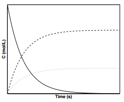
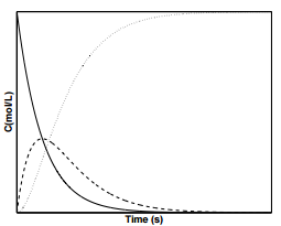
Figure $\PageIndex{2}$ displays the concentration profiles for species $\text{A}$, $\text{I}$, and $\text{P}$ in a consecutive reaction in which $k_1 = k_2$. As can be seen from the figure, the concentration of species $\text{I}$ reaches a maximum at some time, $t_\text{max}$. Oftentimes, species $\text{I}$ is the desired product. Returning to the oxidation of ethylene into ethylene oxide, it is important to note another reaction in which ethylene oxide can decompose into carbon dioxide and water through the following reaction

$$C_2 H_4 O + \dfrac{5}{2} \: O_2 \overset{k_3}{\longrightarrow} 2 \: CO_2 + 2 \: H_2 O$$

Thus, to maximize the concentration of ethylene oxide, the oxidation of ethylene is only allowed proceed to partial completion before the reaction is stopped.

Finally, in the limiting case when $k_2 \gg k_1$, we can write the concentration of $\text{P}$ as

$$\left[ \text{P} \right] \approx \left[ \text{A} \right]_0 \left\{ 1 + \dfrac{1}{-k_2} k_2 e^{-k_1 t} \right\} = \left[ \text{A} \right]_0 \left( 1 - e^{-k_1 t} \right) \label{21.15}$$

Thus, when $k_2 \gg k_1$, the reaction can be approximated as $\text{A} \rightarrow \text{P}$ and the apparent rate law follows $1^{st}$ order kinetics.

Figure $\PageIndex{2}$: Plots of $\left[ \text{A} \right]$ (solid line), $\left[ \text{I} \right]$ (dashed line) and $\left[ \text{P} \right]$ (dotted line) over time for consecutive first order reactions.

Consecutive Reactions With an Equilibrium

Consider the reactions

$$\text{A} \overset{k_1}{\underset{k_{-1}}{\rightleftharpoons}} \text{I} \overset{k_2}{\rightarrow} \text{P}$$

We can write the reaction rates as:

$$\dfrac{d \left[ \text{A} \right]}{dt} = -k_1 \left[ \text{A} \right] + k_{-1} \left[ \text{I} \right] \label{21.16}$$

$$\dfrac{d \left[ \text{I} \right]}{dt} = k_1 \left[ \text{A} \right] - k_{-1} \left[ \text{I} \right] - k_2 \left[ \text{I} \right] \label{21.17}$$

$$\dfrac{ d \left[ \text{P} \right]}{dt} = k_2 \left[ \text{I} \right] \label{21.18}$$

The exact solutions of these is straightforward, in principle, but rather involved, so we will just state the exact solutions, which are

$$\begin{align} \left[ \text{A} \right] \left( t \right) &= \dfrac{ \left[ \text{A} \right]_0}{2 \lambda} \left[ \left( \lambda - k_1 + K \right) e^{-\left( k_1 + K - \lambda \right) t/2} + \left( \lambda + k_1 - K \right) e^{-\left( k_1 + K + \lambda \right) t/2} \right] \\ \left[ \text{I} \right] \left( t \right) &= \dfrac{ k_1 \left[ \text{A} \right]_0}{\lambda} \left[ e^{- \left( k_1 + K - \lambda \right) t/2} - e^{-\left( k_1 + K + \lambda \right) t/2} \right] \\ \left[ \text{P} \right] \left( t \right) &= 2 k_1 k_2 \left[ \text{A} \right]_0 \left[ \dfrac{2}{\left( k_1 + K \right)^2 - \lambda^2} - \dfrac{1}{\lambda} \left( \dfrac{ e^{-\left( k_1 + K - \lambda \right) t/2}}{k_1 + K - \lambda} - \dfrac{e^{-\left( k_1 + K + \lambda \right) t/2}}{k_1 + K + \lambda} \right) \right] \end{align} \label{21.19}$$

where

$$\begin{align} K &= k_2 + k_{-1} \\ \lambda &= \sqrt{\left( k_1 - K \right)^2 - 4k_1 k_{-1}} \end{align} \label{21.20}$$

Steady-State Approximations

Consider the following consecutive reaction in which the first step is reversible:

$$\text{A} \overset{k_1}{\underset{k_{-1}}{\rightleftharpoons}} \text{I} \overset{k_2}{\rightarrow} \text{P}$$

We can write the reaction rates as:

$$\dfrac{d \left[ \text{A} \right]}{dt} = -k_1 \left[ \text{A} \right] + k_{-1} \left[ \text{I} \right] \label{21.21}$$

$$\dfrac{ d \left[ \text{I} \right]}{dt} = k_1 \left[ \text{A} \right] - k_{-1} \left[ \text{I} \right] - k_2 \left[ \text{I} \right] \label{21.22}$$

$$\dfrac{d \left[ \text{P} \right]}{dt} = k_2 \left[ \text{I} \right] \label{21.23}$$

These equations can be solved explicitly in terms of $\left[ \text{A} \right]$, $\left[ \text{I} \right]$, and $\left[ \text{P} \right]$, but the math becomes very complicated quickly. If, however, $k_2 + k_{-1} \gg k_1$ (in other words, the rate of consumption of $\text{I}$ is much faster than the rate of production of $\text{I}$), we can make the approximation that the concentration of the intermediate species, $\text{I}$, is small and constant with time:

$$\dfrac{d \left[ \text{I} \right]}{dt} \approx 0 \label{21.24}$$

Equation 21.22 can now be written as

$$\dfrac{d \left[ \text{I} \right]}{dt} = k_1 \left[ \text{A} \right] - k_{-1} \left[ \text{I} \right]_{ss} - k_2 \left[ \text{I} \right]_{ss} \approx 0 \label{21.25}$$

where $\left[ \text{I} \right]_{ss}$ is a constant represents the steady state concentration of intermediate species, $\left[ \text{I} \right]$. Solving for $\left[ \text{I} \right]_{ss}$,

$$\left[ \text{I} \right]_{ss} = \dfrac{k_1}{k_{-1} + k_2} \left[ \text{A} \right] \label{21.26}$$

We can then write the rate equation for species $\text{A}$ as

$$\dfrac{d \left[ \text{A} \right]}{dt} = -k_1 \left[ \text{A} \right] + k_{-1} \left[ \text{I} \right]_{ss} = -k_1 \left[ \text{A} \right] + k_{-1} \dfrac{k_1}{k_{-1} + k_2} \left[ \text{A} \right] = -\dfrac{k_1 k_2}{k_{-1} + k_2} \left[ \text{A} \right] \label{21.27}$$

Integrating,

$$\left[ \text{A} \right] = \left[ \text{A} \right]_0 e^{-\dfrac{k_1 k_2}{k_{-1} + k_2} t} \label{21.28}$$

Equation 21.28 is the same equation we would obtain for apparent $1^{st}$ order kinetics of the following reaction:

$$\text{A} \overset{k'}{\longrightarrow} \text{P}$$

where

$$k' = \dfrac{k_1 k_2}{k_{-1} + k_2} \label{21.29}$$

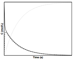
Figure $\PageIndex{3}$ displays the concentration profiles for species, $\text{A}$, $\text{I}$, and $\text{P}$ with the condition that $k_2 + k_{-1} \gg k_1$. These types of reaction kinetics appear when the intermediate species, $\text{I}$, is highly reactive.

Figure $\PageIndex{3}$: Plots of $\left[ \text{A} \right]$ (solid line), $\left[ \text{I} \right]$ (dashed line) and $\left[ \text{P} \right]$ (dotted line) over time for $k_2 + k_{-1} \gg k_1$.

Lindemann Mechanism

Consider the isomerization of methylisonitrile gas, $CH_3 NC$, to acetonitrile gas, $CH_3 CN$:

$$CH_3 NC \overset{k}{\longrightarrow} CH_3 CN$$

If the isomerization is a unimolecular elementary reaction, we should expect to see $1^{st}$ order rate kinetics. Experimentally, however, $1^{st}$ order rate kinetics are only observed at high pressures. At low pressures, the reaction kinetics follow a $2^{nd}$ order rate law:

$$\dfrac{d \left[ CH_3 NC \right]}{dt} = -k \left[ CH_3 NC \right]^2 \label{21.30}$$

To explain this observation, J.A. Christiansen and F.A. Lindemann proposed that gas molecules first need to be energized via intermolecular collisions before undergoing an isomerization reaction. The reaction mechanism can be expressed as the following two elementary reactions

$$\begin{align} \text{A} + \text{M} &\overset{k_1}{\underset{k_{-1}}{\rightleftharpoons}} \text{A}^* + \text{M} \\ \text{A}^* &\overset{k_2}{\rightarrow} \text{B} \end{align}$$

where $\text{M}$ can be a reactant molecule, a product molecule or another inert molecule present in the reactor. Assuming that the concentration of $\text{A}^*$ is small, or $k_1 \ll k_2 + k_{-1}$, we can use a steady-state approximation to solve for the concentration profile of species $\text{B}$ with time:

$$\dfrac{d \left[ \text{A}^* \right]}{dt} = k_1 \left[ \text{A} \right] \left[ \text{M} \right] - k_{-1} \left[ \text{A}^* \right]_{ss} \left[ \text{M} \right] - k_2 \left[ \text{A}^* \right]_{ss} \approx 0 \label{21.31}$$

Solving for $\left[ \text{A}^* \right]$,

$$\left[ \text{A}^* \right] = \dfrac{k_1 \left[ \text{M} \right] \left[ \text{A} \right]}{k_2 + k_{-1} \left[ \text{M} \right]} \label{21.32}$$

The reaction rates of species $\text{A}$ and $\text{B}$ can be written as

$$-\dfrac{d \left[ \text{A} \right]}{dt} = \dfrac{d \left[ \text{B} \right]}{dt} = k_2 \left[ \text{A}^* \right] = \dfrac{k_1 k_2 \left[ \text{M} \right] \left[ \text{A} \right]}{k_2 + k_{-1} \left[ \text{M} \right]} = k_\text{obs} \left[ \text{A} \right] \label{21.33}$$

where

$$k_\text{obs} = \dfrac{k_1 k_2 \left[ \text{M} \right]}{k_2 + k_{-1} \left[ \text{M} \right]} \label{21.34}$$

At high pressures, we can expect collisions to occur frequently, such that $k_{-1} \left[ \text{M} \right] \gg k_2$. Equation 21.33 then becomes

$$-\dfrac{d \left[ \text{A} \right]}{dt} = \dfrac{k_1 k_2}{k_{-1}} \left[ \text{A} \right] \label{21.35}$$

which follows $1^{st}$ order rate kinetics.

At low pressures, we can expect collisions to occurs infrequently, such that $k_{-1} \left[ \text{M} \right] \ll k_2$. In this scenario, equation 21.33 becomes

$$-\dfrac{d \left[ \text{A} \right]}{dt} = k_1 \left[ \text{A} \right] \left[ \text{M} \right] \label{21.36}$$

which follows second order rate kinetics, consistent with experimental observations.

Equilibrium Approximations

Consider again the following consecutive reaction in which the first step is reversible:

$$\text{A} \overset{k_1}{\underset{k_{-1}}{\rightleftharpoons}} \text{I} \overset{k_2}{\rightarrow} \text{P}$$

Now let us consider the situation in which $k_2 \ll k_1$ and $k_{-1}$. In other words, the conversion of $\text{I}$ to $\text{P}$ is slow and is the rate-limiting step. In this situation, we can assume that $\left[ \text{A} \right]$ and $\left[ \text{I} \right]$ are in equilibrium with each other. As we derived before for a reversible reaction in equilibrium,

$$K_\text{eq} = \dfrac{k_1}{k_{-1}} \approx \dfrac{ \left[ \text{I} \right]}{\left[ \text{A} \right]} \label{21.37}$$

or, in terms of $\left[ \text{I} \right]$,

$$\left[ \text{I} \right] = K_\text{eq} \left[ \text{A} \right] \label{21.38}$$

These conditions also result from the exact solution when we set $k_2 \approx 0$. When this is done, we have the approximate expressions from the exact solution:

$$\begin{align} K &\approx k_{-1} \\ \lambda &\approx \sqrt{ \left( k_1 - k_{-1} \right)^2 + 4k_1 k_{-1}} = \sqrt{k_1^2 + 2k_1 k_{-1} + k_{-1}^2} = k_1 + k_{-1} \\ \lambda - k_1 + K &\approx k_1 + k_{-1} + k_1 - k_{-1} = 2k_1 \\ \lambda + k_1 - K &\approx k_1 + k_{-1} + k_1 - k_{-1} = 2k_1 \\ k_1 + K - \lambda &\approx k_1 + k_{-1} - k_1 - k_{-1} = 0 \\ k_1 + K + \lambda &\approx k_1 + k_{-1} + k_1 + k_{-1} = 2 \left( k_1 + k_{-1} \right) \end{align} \label{21.39}$$

and the approximate solutions become

$$\begin{align} \left[ \text{A} \right] \left( t \right) &= \dfrac{ \left[ \text{A} \right]_0}{2 \left( k_1 + k_{-1} \right)} \left[ 2k_{-1} + 2k_1 e^{-\left( k_1 + k_{-1} \right) t} \right] \\ \left[ \text{I} \right] \left( t \right) &= \dfrac{k_1 \left[ \text{A} \right]_0}{\left( k_1 + k_{-1} \right)} \left[ 1 - e^{-\left( k_1 + k_{-1} \right) t} \right] \end{align} \label{21.40}$$

In the long-time limit, when equilibrium is reached and transient behavior has decayed away, we find

$$\dfrac{ \left[ \text{I} \right]}{\left[ \text{A} \right]} \equiv K_\text{eq} \rightarrow \dfrac{k_1}{k_{-1}} \label{21.41}$$

Plugging the above equation into the expression for $d \left[ \text{P} \right]/dt$,

$$\dfrac{d \left[ \text{P} \right]}{dt} = k_2 \left[ \text{I} \right] = k_2 K_\text{eq} \left[ \text{A} \right] = \dfrac{k_1 k_2}{k_{-1}} \left[ \text{A} \right] \label{21.42}$$

The reaction can thus be approximated as a $1^{st}$ order reaction

$$\text{A} \overset{k'}{\longrightarrow} \text{P}$$

with

$$k' = \dfrac{k_1 k_2}{k_{-1}} \label{21.43}$$

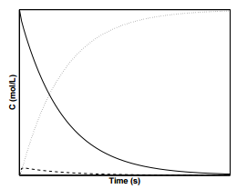
Figure $\PageIndex{4}$ displays the concentration profiles for species, $\text{A}$, $\text{I}$, and $\text{P}$ with the condition that $k_2 \ll k_1 = k_{-1}$. When $k_1 = k_{-1}$, we expect $\left[ \text{A} \right] = \left[ \text{I} \right]$. As can be seen from the figure, after a short initial startup time, the concentrations of species $\text{A}$ and $\text{I}$ are approximately equal during the reaction.

Figure $\PageIndex{4}$: Plots of $\left[ \text{A} \right]$ (solid line), $\left[ \text{I} \right]$ (dashed line) and $\left[ \text{P} \right]$ (dotted line) over time for $k_2 \ll k_1 = k_{-1}$.