8.2: Reaction Order

The kinetic theory of gases can be used to model the frequency of collisions between hard-sphere molecules, which is proportional to the reaction rate. Most systems undergoing a chemical reaction, however, are much more complex. The reaction rates may be dependent on specific interactions between reactant molecules, the phase(s) in which the reaction takes place, etc. The field of chemical kinetics is thus by-and-large based on empirical observations. From experimental observations, scientists have established that reaction rates almost always have a power-law dependence on the concentrations of one or more of the reactants. In the following sections, we will discuss different power laws that are commonly observed in chemical reactions.

$0^{th}$ Order Reaction Kinetics

Consider a closed container initially filled with chemical species $A$. At $t = 0$, a stimulus, such as a change in temperature, the addition of a catalyst, or irradiation, causes an irreversible chemical reaction to occur in which $A$ transforms into product $B$:

$$a \text{A} \longrightarrow b \text{B}$$

The rate that the reaction proceeds, $r$, can be described as the change in the concentrations of the chemical species with respect to time:

$$r = -\dfrac{1}{a} \dfrac{d \left[ \text{A} \right]}{dt} = \dfrac{1}{b} \dfrac{d \left[ \text{B} \right]}{dt} \label{19.1}$$

where $\left[ \text{X} \right]$ denotes the molar concentration of chemical species $\text{X}$ with units of $\frac{\text{mol}}{\text{L}^3}$.

Let us first examine a reaction $\text{A} \longrightarrow \text{B}$ in which the reaction rate, $r$, is constant with time:

$$r = -\dfrac{d \left[ \text{A} \right]}{dt} = k \label{19.2}$$

where $k$ is a constant, also known as the rate constant with units of $\dfrac{\text{mol}}{\text{m}^3 \text{s}}$. Such reactions are called zeroth order reactions because the reaction rate depends on the concentrations of species $\text{A}$ and $\text{B}$ to the $0^{th}$ power. Integrating $\left[ \text{A} \right]$ with respect to $T$, we find that

$$\left[ \text{A} \right] = -kt + c_1 \label{19.3}$$

At $t = 0$, $\left[ \text{A} \right] \left( 0 \right) = \left[ \text{A} \right]_0$. Plugging these values into the equation, we find that $c_1 = \left[ \text{A} \right]_0$. The final form of the equation is:

$$\left[ \text{A} \right] = \left[ \text{A} \right]_0 - kt \label{19.4}$$

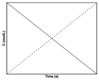
A plot of the concentration of species $\text{A}$ with time for a $0^{th}$ order reaction is shown in Figure $\PageIndex{1}$, where the slope of the line is $-k$ and the $y$-intercept is $\left[ \text{A} \right]_0$. Such reactions in which the reaction rates are independent of the concentrations of products and reactants are rare in nature. An example of a system displaying $0^{th}$ order kinetics would be one in which a reaction is mediated by a catalyst present in small amounts.

$1^{st}$ Order Reaction Kinetics

Experimentally, it is observed than when a chemical reaction is of the form

$$\sum_i \nu_i \text{A}_i = 0 \label{19.5}$$

the reaction rate can be expressed as

$$r = k \prod_\text{reactants} \left[ \text{A}_i \right]^{\nu_i} \label{19.6}$$

where it is assumed that the stoichiometric coefficients $\nu_i$ of the reactants are all positive. Thus, or a reaction $\text{A} \longrightarrow \text{B}$, the reaction rate depends on $\left[ \text{A} \right]$ raised to the first power:

$$r = \dfrac{d \left[ \text{A} \right]}{dt} = -k \left[ \text{A} \right] \label{19.7}$$

Figure $\PageIndex{1}$: Plots of $\left[ \text{A} \right]$ (solid line) and $\left[ \text{B} \right]$ (dashed line) over time for a $0^{th}$ order reaction.

For first order reactions, $k$ has the units of $\dfrac{1}{\text{s}}$. Integrating and applying the condition that at $t = 0 \: \text{s}$, $\left[ \text{A} \right] = \left[ \text{A} \right]_0$, we arrive at the following equation:

$$\left[ \text{A} \right] = \left[ \text{A} \right] e^{-kt} \label{19.8}$$

Figure $\PageIndex{2}$ displays the concentration profiles for species $\text{A}$ and $\text{B}$ for a first order reaction. To determine the value of $k$ from

Figure $\PageIndex{2}$: Plots of $\left[ \text{A} \right]$ (solid line) and $\left[ \text{B} \right]$ (dashed line) over time for a $1^{st}$ order reaction.

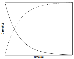
experimental data, it is convenient to take the natural log of Equation $\ref{19.8}$:

$$\text{ln} \left( \left[ \text{A} \right] \right) = \text{ln} \left( \left[ \text{A} \right]_0 \right) - kt \label{19.9}$$

For a first order irreversible reaction, a plot of $\text{ln} \left( \left[ \text{A} \right] \right)$ vs. $t$ is straight line with a slope of $-k$ and a $y$-intercept of $\text{ln} \left( \left[ \text{A} \right]_0 \right)$.

$2^{nd}$ Order Reaction Kinetics

Another type of reaction depends on the square of the concentration of species $\text{A}$ - these are known as second order reactions. For a second order reaction in which $2 \text{A} \longrightarrow \text{B}$, we can write the reaction rate to be

$$r = -\dfrac{1}{2} \dfrac{d \left[ \text{A} \right]}{dt} = k \left[ \text{A} \right]^2 \label{19.10}$$

For second order reactions, $k$ has the units of $\dfrac{\text{m}^3}{\text{mol} \cdot \text{s}}$. Integrating and applying the condition that at $t = 0 \: \text{s}$, $\left[ \text{A} \right] = \left[ \text{A} \right]_0$, we arrive at the following equation for the concentration of $\text{A}$ over time:

$$\left[ \text{A} \right] = \dfrac{1}{2kt + \dfrac{1}{\left[ \text{A} \right]_0}} \label{19.11}$$

Figure $\PageIndex{3}$ shows concentration profiles of $\text{A}$ and $\text{B}$ for a second order reaction. To determine $k$ from experimental data for

Figure $\PageIndex{3}$: Plots of $\left[ \text{A} \right]$ (solid line) and $\left[ \text{B} \right]$ (dashed line) over time for a $2^{nd}$ order reaction.

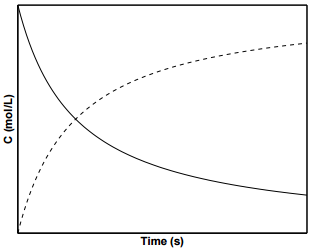
second-order reactions, it is convenient to invert Equation $\ref{19.11}$:

$$\dfrac{1}{\left[ \text{A} \right]} = \dfrac{1}{\left[ \text{A} \right]_0} + 2kt \label{19.12}$$

A plot of $1/\left[ \text{A} \right]$ vs. $t$ will give rise to a straight line with slope $k$ and intercept $1/\left[ \text{A} \right]_0$.

Second order reaction rates can also apply to reactions in which two species react with each other to form a product:

$$\text{A} + \text{B} \overset{k}{\longrightarrow} \text{C}$$

In this scenario, the reaction rate will depend on the concentrations of both $\text{A}$ and $\text{B}$ to the first order:

$$r = -\dfrac{d \left[ \text{A} \right]}{dt} = -\dfrac{d \left[ \text{B} \right]}{dt} = k \left[ \text{A} \right] \left[ \text{B} \right] \label{19.13}$$

To integrate the above equation, we need to write it in terms of one variable. Since the concentrations of $\text{A}$ and $\text{B}$ are related to each other via the chemical reaction equation, we can write:

$$\left[ \text{B} \right] = \left[ \text{B} \right]_0 - \left( \left[ \text{A} \right]_0 - \left[ \text{A} \right] \right) = \left[ \text{A} \right] + \left[ \text{B} \right]_0 - \left[ \text{A} \right]_0 \label{19.14}$$

$$\dfrac{d \left[ \text{A} \right]}{dt} = -k \left[ \text{A} \right] \left( \left[ \text{A} \right] + \left[ \text{B} \right]_0 - \left[ \text{A} \right]_0 \right) \label{19.15}$$

We can then use partial fractions to integrate:

$$kdt = \dfrac{d \left[ \text{A} \right]}{\left[ \text{A} \right] \left( \left[ \text{A} \right] + \left[ \text{B} \right]_0 - \left[ \text{A} \right]_0 \right)} = \dfrac{1}{\left[ \text{B} \right]_0 - \left[ \text{A} \right]_0} \left( \dfrac{d \left[ \text{A} \right]}{\left[ \text{A} \right]} - \dfrac{d \left[ \text{A} \right]}{\left[ \text{B} \right]_0 - \left[ \text{A} \right]_0 + \left[ \text{A} \right]} \right) \label{19.16}$$

$$kt = \dfrac{1}{\left[ \text{A} \right]_0 - \left[ \text{B} \right]_0} \text{ln} \dfrac{\left[ \text{A} \right] \left[ \text{B} \right]_0}{\left[ \text{B} \right] \left[ \text{A} \right]_0} \label{19.17}$$

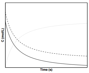
Figure $\PageIndex{4}$ displays the concentration profiles of species $\text{A}$, $\text{B}$, and $\text{C}$ for a second order reaction in which the initial concentrations of $\text{A}$ and $\text{B}$ are not equal.

Figure $\PageIndex{4}$: Plots of $\left[ \text{A} \right]$ (solid line), $\left[ \text{B} \right]$ (dashed line) and $\left[ \text{C} \right]$ (dotted line) over time for a $2^{nd}$ order reaction in which the initial concentrations of the reactants, $\left[ \text{A} \right]_0$ and $\left[ \text{B} \right]_0$, are not equal.

Contributors

• Mark Tuckerman (New York University)