
1.9: More on Kinetic Molecular Theory
- Page ID
- 152846

\( \newcommand{\vecs}[1]{\overset { \scriptstyle \rightharpoonup} {\mathbf{#1}} } \)
\( \newcommand{\vecd}[1]{\overset{-\!-\!\rightharpoonup}{\vphantom{a}\smash {#1}}} \)
\( \newcommand{\id}{\mathrm{id}}\) \( \newcommand{\Span}{\mathrm{span}}\)
( \newcommand{\kernel}{\mathrm{null}\,}\) \( \newcommand{\range}{\mathrm{range}\,}\)
\( \newcommand{\RealPart}{\mathrm{Re}}\) \( \newcommand{\ImaginaryPart}{\mathrm{Im}}\)
\( \newcommand{\Argument}{\mathrm{Arg}}\) \( \newcommand{\norm}[1]{\| #1 \|}\)
\( \newcommand{\inner}[2]{\langle #1, #2 \rangle}\)
\( \newcommand{\Span}{\mathrm{span}}\)
\( \newcommand{\id}{\mathrm{id}}\)
\( \newcommand{\Span}{\mathrm{span}}\)
\( \newcommand{\kernel}{\mathrm{null}\,}\)
\( \newcommand{\range}{\mathrm{range}\,}\)
\( \newcommand{\RealPart}{\mathrm{Re}}\)
\( \newcommand{\ImaginaryPart}{\mathrm{Im}}\)
\( \newcommand{\Argument}{\mathrm{Arg}}\)
\( \newcommand{\norm}[1]{\| #1 \|}\)
\( \newcommand{\inner}[2]{\langle #1, #2 \rangle}\)
\( \newcommand{\Span}{\mathrm{span}}\) \( \newcommand{\AA}{\unicode[.8,0]{x212B}}\)
\( \newcommand{\vectorA}[1]{\vec{#1}} % arrow\)
\( \newcommand{\vectorAt}[1]{\vec{\text{#1}}} % arrow\)
\( \newcommand{\vectorB}[1]{\overset { \scriptstyle \rightharpoonup} {\mathbf{#1}} } \)
\( \newcommand{\vectorC}[1]{\textbf{#1}} \)
\( \newcommand{\vectorD}[1]{\overrightarrow{#1}} \)
\( \newcommand{\vectorDt}[1]{\overrightarrow{\text{#1}}} \)
\( \newcommand{\vectE}[1]{\overset{-\!-\!\rightharpoonup}{\vphantom{a}\smash{\mathbf {#1}}}} \)
\( \newcommand{\vecs}[1]{\overset { \scriptstyle \rightharpoonup} {\mathbf{#1}} } \)
\( \newcommand{\vecd}[1]{\overset{-\!-\!\rightharpoonup}{\vphantom{a}\smash {#1}}} \)
\(\newcommand{\avec}{\mathbf a}\) \(\newcommand{\bvec}{\mathbf b}\) \(\newcommand{\cvec}{\mathbf c}\) \(\newcommand{\dvec}{\mathbf d}\) \(\newcommand{\dtil}{\widetilde{\mathbf d}}\) \(\newcommand{\evec}{\mathbf e}\) \(\newcommand{\fvec}{\mathbf f}\) \(\newcommand{\nvec}{\mathbf n}\) \(\newcommand{\pvec}{\mathbf p}\) \(\newcommand{\qvec}{\mathbf q}\) \(\newcommand{\svec}{\mathbf s}\) \(\newcommand{\tvec}{\mathbf t}\) \(\newcommand{\uvec}{\mathbf u}\) \(\newcommand{\vvec}{\mathbf v}\) \(\newcommand{\wvec}{\mathbf w}\) \(\newcommand{\xvec}{\mathbf x}\) \(\newcommand{\yvec}{\mathbf y}\) \(\newcommand{\zvec}{\mathbf z}\) \(\newcommand{\rvec}{\mathbf r}\) \(\newcommand{\mvec}{\mathbf m}\) \(\newcommand{\zerovec}{\mathbf 0}\) \(\newcommand{\onevec}{\mathbf 1}\) \(\newcommand{\real}{\mathbb R}\) \(\newcommand{\twovec}[2]{\left[\begin{array}{r}#1 \\ #2 \end{array}\right]}\) \(\newcommand{\ctwovec}[2]{\left[\begin{array}{c}#1 \\ #2 \end{array}\right]}\) \(\newcommand{\threevec}[3]{\left[\begin{array}{r}#1 \\ #2 \\ #3 \end{array}\right]}\) \(\newcommand{\cthreevec}[3]{\left[\begin{array}{c}#1 \\ #2 \\ #3 \end{array}\right]}\) \(\newcommand{\fourvec}[4]{\left[\begin{array}{r}#1 \\ #2 \\ #3 \\ #4 \end{array}\right]}\) \(\newcommand{\cfourvec}[4]{\left[\begin{array}{c}#1 \\ #2 \\ #3 \\ #4 \end{array}\right]}\) \(\newcommand{\fivevec}[5]{\left[\begin{array}{r}#1 \\ #2 \\ #3 \\ #4 \\ #5 \\ \end{array}\right]}\) \(\newcommand{\cfivevec}[5]{\left[\begin{array}{c}#1 \\ #2 \\ #3 \\ #4 \\ #5 \\ \end{array}\right]}\) \(\newcommand{\mattwo}[4]{\left[\begin{array}{rr}#1 \amp #2 \\ #3 \amp #4 \\ \end{array}\right]}\) \(\newcommand{\laspan}[1]{\text{Span}\{#1\}}\) \(\newcommand{\bcal}{\cal B}\) \(\newcommand{\ccal}{\cal C}\) \(\newcommand{\scal}{\cal S}\) \(\newcommand{\wcal}{\cal W}\) \(\newcommand{\ecal}{\cal E}\) \(\newcommand{\coords}[2]{\left\{#1\right\}_{#2}}\) \(\newcommand{\gray}[1]{\color{gray}{#1}}\) \(\newcommand{\lgray}[1]{\color{lightgray}{#1}}\) \(\newcommand{\rank}{\operatorname{rank}}\) \(\newcommand{\row}{\text{Row}}\) \(\newcommand{\col}{\text{Col}}\) \(\renewcommand{\row}{\text{Row}}\) \(\newcommand{\nul}{\text{Nul}}\) \(\newcommand{\var}{\text{Var}}\) \(\newcommand{\corr}{\text{corr}}\) \(\newcommand{\len}[1]{\left|#1\right|}\) \(\newcommand{\bbar}{\overline{\bvec}}\) \(\newcommand{\bhat}{\widehat{\bvec}}\) \(\newcommand{\bperp}{\bvec^\perp}\) \(\newcommand{\xhat}{\widehat{\xvec}}\) \(\newcommand{\vhat}{\widehat{\vvec}}\) \(\newcommand{\uhat}{\widehat{\uvec}}\) \(\newcommand{\what}{\widehat{\wvec}}\) \(\newcommand{\Sighat}{\widehat{\Sigma}}\) \(\newcommand{\lt}{<}\) \(\newcommand{\gt}{>}\) \(\newcommand{\amp}{&}\) \(\definecolor{fillinmathshade}{gray}{0.9}\)Skills to Develop
Make sure you thoroughly understand the following essential ideas that are presented below. It is especially important that you know the precise meanings of all the italicized terms in the context of this topic.
- You should be able to sketch the general shape of the Maxwell-Boltzmann plot showing the distribution of molecular velocities. You should also show how these plots are affected by the temperature and by the molar mass.
- Although there is no need for you to be able to derive the ideal gas equation of state, you should understand that the equation PV = nRTcan be derived from the principles of kinetic molecular theory, as outlined above.
- Explain the concept of the mean free path of a gas molecule (but no need to reproduce the mathematics.)
In this section, we look in more detail at some aspects of the kinetic-molecular model and how it relates to our empirical knowledge of gases. For most students, this will be the first application of algebra to the development of a chemical model; this should be educational in itself, and may help bring that subject back to life for you! As before, your emphasis should on understanding these models and the ideas behind them, there is no need to memorize any of the formulas.
The velocities of gas molecules
At temperatures above absolute zero, all molecules are in motion. In the case of a gas, this motion consists of straight-line jumps whose lengths are quite great compared to the dimensions of the molecule. Although we can never predict the velocity of a particular individual molecule, the fact that we are usually dealing with a huge number of them allows us to know what fraction of the molecules have kinetic energies (and hence velocities) that lie within any given range.
The trajectory of an individual gas molecule consists of a series of straight-line paths interrupted by collisions. What happens when two molecules collide depends on their relative kinetic energies; in general, a faster or heavier molecule will impart some of its kinetic energy to a slower or lighter one. Two molecules having identical masses and moving in opposite directions at the same speed will momentarily remain motionless after their collision.
If we could measure the instantaneous velocities of all the molecules in a sample of a gas at some fixed temperature, we would obtain a wide range of values. A few would be zero, and a few would be very high velocities, but the majority would fall into a more or less well defined range. We might be tempted to define an average velocity for a collection of molecules, but here we would need to be careful: molecules moving in opposite directions have velocities of opposite signs. Because the molecules are in a gas are in random thermal motion, there will be just about as many molecules moving in one direction as in the opposite direction, so the velocity vectors of opposite signs would all cancel and the average velocity would come out to zero. Since this answer is not very useful, we need to do our averaging in a slightly different way.
The proper treatment is to average the squares of the velocities, and then take the square root of this value. The resulting quantity is known as the root mean square, or RMS velocity
\[ \nu_{rms} = \sqrt{\dfrac{\sum \nu^2}{n}}\]
which we will denote simply by \(\bar{v}\). The formula relating the RMS velocity to the temperature and molar mass is surprisingly simple, considering the great complexity of the events it represents:
\[ \bar{v}= v_{rms} = \sqrt{\dfrac{3RT}{m}}\]
in which m is the molar mass in kg mol–1, and k = R÷6.02E23, the “gas constant per molecule", is known as the Boltzmann constant.
Example 6.5.1
What is the average velocity of a nitrogen molecules at 300 K?
SOLUTION
The molar mass of N2 is 28.01 g. Substituting in the above equation and expressing R in energy units, we obtain
Recalling the definition of the joule (1 J = 1 kg m2 s–2) and taking the square root,
or
Comment: this is fast! The velocity of a rifle bullet is typically 300-500 m s–1; convert to common units to see the comparison for yourself.
A simpler formula for estimating average molecular velocities is
\[v=157 \sqrt{\dfrac{T}{m}}\]
in which \(v\) is in units of meters/sec, \(T\) is the absolute temperature and \(m\) the molar mass in grams.
The Boltzmann Distribution
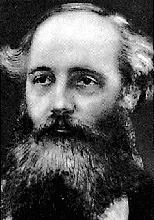
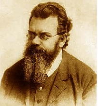
If we were to plot the number of molecules whose velocities fall within a series of narrow ranges, we would obtain a slightly asymmetric curve known as a velocity distribution. The peak of this curve would correspond to the most probable velocity. This velocity distribution curve is known as the Maxwell-Boltzmann distribution, but is frequently referred to only by Boltzmann's name. The Maxwell-Boltzmann distribution law was first worked out around 1850 by the great Scottish physicist, James Clerk Maxwell (left, 1831-1879), who is better known for discovering the laws of electromagnetic radiation. Later, the Austrian physicist Ludwig Boltzmann (1844-1906) put the relation on a sounder theoretical basis and simplified the mathematics somewhat. Boltzmann pioneered the application of statistics to the physics and thermodynamics of matter, and was an ardent supporter of the atomic theory of matter at a time when it was still not accepted by many of his contemporaries.
The derivation of the Boltzmann curve is a bit too complicated to go into here, but its physical basis is easy to understand. Consider a large population of molecules having some fixed amount of kinetic energy. As long as the temperature remains constant, this total energy will remain unchanged, but it can be distributed among the molecules in many different ways, and this distribution will change continually as the molecules collide with each other and with the walls of the container.
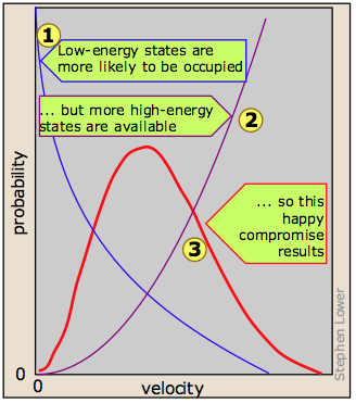
It turns out, however, that kinetic energy is acquired and handed around only in discrete amounts which are known as quanta. Once the molecule has a given number of kinetic energy quanta, these can be apportioned amongst the three directions of motion in many different ways, each resulting in a distinct total velocity state for the molecule. The greater the number of quanta, (that is, the greater the total kinetic energy of the molecule) the greater the number of possible velocity states. If we assume that all velocity states are equally probable, then simple statistics predicts that higher velocities will be more favored simply because there are so many more of them  .
.
Although the number of possible higher-energy states is greater, the lower-energy states are more likely to be occupied  . This is because only so much kinetic energy available to the gas as a whole; every molecule that acquires kinetic energy in a collision leaves behind another molecule having less. This tends to even out the kinetic energies in a collection of molecules, and ensures that there are always some molecules whose instantaneous velocity is near zero. The net effect of these two opposing tendencies, one favoring high kinetic energies and the other favoring low ones, is the peaked curve
  seen above. Notice that because of the asymmetry of this curve, the mean (rms average) velocity is not the same as the most probable velocity, which is defined by the peak of the curve.
At higher temperatures (or with lighter molecules) the latter constraint becomes less important, and the mean velocity increases. But with a wider velocity distribution, the number of molecules having any one velocity diminishes, so the curve tends to flatten out.
Velocity Distributions Depend on Temperature and Mass
Higher temperatures allow a larger fraction of molecules to acquire greater amounts of kinetic energy, causing the Boltzmann plots to spread out.
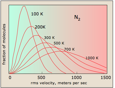
Notice how the left ends of the plots are anchored at zero velocity (there will always be a few molecules that happen to be at rest.) As a consequence, the curves flatten out as the higher temperatures make additional higher-velocity states of motion more accessible. The area under each plot is the same for a constant number of molecules.
All molecules have the same kinetic energy (mv2/2) at the same temperature, so the fraction of molecules with higher velocities will increase as m, and thus the molecular weight, decreases.
Boltzmann Distribution and Planetary Atmospheres
The ability of a planet to retain an atmospheric gas depends on the average velocity (and thus on the temperature and mass) of the gas molecules and on the planet's mass, which determines its gravity and thus the escape velocity. In order to retain a gas for the age of the solar system, the average velocity of the gas molecules should not exceed about one-sixth of the escape velocity. The escape velocity from the Earth is 11.2 km/s, and 1/6 of this is about 2 km/s. Examination of the above plot reveals that hydrogen molecules can easily achieve this velocity, and this is the reason that hydrogen, the most abundant element in the universe, is almost absent from Earth's atmosphere.
Although hydrogen is not a significant atmospheric component, water vapor is. A very small amount of this diffuses to the upper part of the atmosphere, where intense solar radiation breaks down the H2O into H2. Escape of this hydrogen from the upper atmosphere amounts to about 2.5 × 10¹⁰ g/year.
Derivation of the Ideal Gas Equation
The ideal gas equation of state came about by combining the empirically determined ("ABC") laws of Avogadro, Boyle, and Charles, but one of the triumphs of the kinetic molecular theory was the derivation of this equation from simple mechanics in the late nineteenth century. This is a beautiful example of how the principles of elementary mechanics can be applied to a simple model to develop a useful description of the behavior of macroscopic matter. We begin by recalling that the pressure of a gas arises from the force exerted when molecules collide with the walls of the container. This force can be found from Newton's law
\[f = ma = m\dfrac{dv}{dt} \label{2.1}\]
in which \(v\) is the velocity component of the molecule in the direction perpendicular to the wall and \(m\) is its mass.
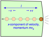
To evaluate the derivative, which is the velocity change per unit time, consider a single molecule of a gas contained in a cubic box of length l. For simplicity, assume that the molecule is moving along the x-axis which is perpendicular to a pair of walls, so that it is continually bouncing back and forth between the same pair of walls. When the molecule of mass m strikes the wall at velocity +v (and thus with a momentum mv ) it will rebound elastically and end up moving in the opposite direction with –v. The total change in velocity per collision is thus 2v and the change in momentum is \(2mv\).
The Frequency of Collisions
After the collision the molecule must travel a distance l to the opposite wall, and then back across this same distance before colliding again with the wall in question. This determines the time between successive collisions with a given wall; the number of collisions per second will be \(v/2l\). The force \(F\) exerted on the wall is the rate of change of the momentum, given by the product of the momentum change per collision and the collision frequency:
\[F = \dfrac{d(mv_x}{dt} = (2mv_x) \times \left( \dfrac{v_x}{2l} \right) = \dfrac{m v_x^2}{l} \label{2-2}\]
Pressure is force per unit area, so the pressure \(P\) exerted by the molecule on the wall of cross-section \(l^2\) becomes
\[ P = \dfrac{mv^2}{l^3} = \dfrac{mv^2}{V} \label{2-3}\]
in which \(V\) is the volume of the box.
The pressure produced by N molecules
As noted near the beginning of this unit, any given molecule will make about the same number of moves in the positive and negative directions, so taking a simple average would yield zero. To avoid this embarrassment, we square the velocities before averaging them, and then take the square root of the average. This result is known as the root mean square (rms) velocity.
We have calculated the pressure due to a single molecule moving at a constant velocity in a direction perpendicular to a wall. If we now introduce more molecules, we must interpret \(v^2\) as an average value which we will denote by \(\bar{v^2}\). Also, since the molecules are moving randomly in all directions, only one-third of their total velocity will be directed along any one cartesian axis, so the total pressure exerted by N molecules becomes
\[ P=\dfrac{N}{3}\dfrac{m \bar{\nu}^2}{V} \label{2.4}\]
The translational kinetic energy
Recalling that mv2/2 is the average translational kinetic energy ε, we can rewrite the above expression as
\[PV = \dfrac{1}{3} N m \bar{v^2} = \dfrac{2}{3} N \epsilon \label{2-5}\]
Relating kinetic energy to the temperature
The 2/3 factor in the proportionality reflects the fact that velocity components in each of the three directions contributes ½ kT to the kinetic energy of the particle. The average translational kinetic energy is directly proportional to temperature:
\[\epsilon = \dfrac{3}{2} kT \label{2.6}\]
in which the proportionality constant k is known as the Boltzmann constant. Substituting this into (2-5) yields
\[ PV = \left( \dfrac{2}{3}N \right) \left( \dfrac{3}{2}kT \right) =NkT \label{2.7}\]
The Boltzmann constant k is just the gas constant per molecule. For n moles of particles, the above equation becomes
\[ P V = n R T \label{2.8}\]
.. and we're home!
RT has the dimensions of energy
Since the product PV has the dimensions of energy, so does RT, and this quantity in fact represents the average translational kinetic energy per mole of molecular particles. The relationship between these two energy units can be obtained by recalling that 1 atm is \(1.013\times 10^{5}\, N\, m^{–2}\), so that
The gas constant R is one of the most important fundamental constants relating to the macroscopic behavior of matter. It is commonly expressed in both pressure-volume and in energy units:
R = 0.082057 L atm mol–1 K–1 = 8.314 J mol–1 K–1
That is, R expresses the amount of energy per Kelvin degree. As noted above, the Boltzmann constant k, which appears in many expressions relating to the statistical treatment of molecules, is just
R ÷ 6.02E23 = 1.3807 × 10⁻²³ J K–1,
the "gas constant per molecule "
How far does a molecule travel between collisions?
Molecular velocities tend to be very high by our everyday standards (typically around 500 meters per sec), but even in gases, they bump into each other so frequently that their paths are continually being deflected in a random manner, so that the net movement (diffusion) of a molecule from one location to another occurs rather slowly. How close can two molecules get?
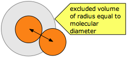
Each molecule is surrounded by an imaginary sphere (gray circle) whose radius \(σ\) is equal to the sum of the radii of the colliding molecules. This sphere defines the excluded volume, within which the center of another molecule cannot enter.
The average distance a molecule moves between such collisions is called the mean free path (\(\lambda\)), which depends on the number of molecules per unit volume and on their size. To avoid collision, a molecule of diameter σ must trace out a path corresponding to the axis of an imaginary cylinder whose cross-section is \(\pi \sigma^2\). Eventually it will encounter another molecule (extreme right in the diagram below) that has intruded into this cylinder and defines the terminus of its free motion.
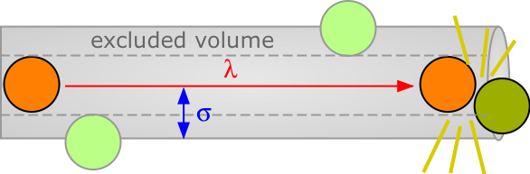
The volume of the cylinder is \(\pi \sigma^2 \lambda.\) At each collision the molecule is diverted to a new path and traces out a new exclusion cylinder. After colliding with all n molecules in one cubic centimeter of the gas it will have traced out a total exclusion volume of \(\pi \sigma^2 \lambda\). Solving for \(\lambda\) and applying a correction factor \(\sqrt{2}\) to take into account exchange of momentum between the colliding molecules (the detailed argument for this is too complicated to go into here), we obtain
\[\lambda = \dfrac{1}{\sqrt{2\pi n \sigma^2}} \label{3.1}\]
Small molecules such as He, H2 and CH4 typically have diameters of around 30-50 pm. At STP the value of \(n\), the number of molecules per cubic meter, is
\[\dfrac{6.022 \times 10^{23}\; mol^{-1}}{22.4 \times 10^{-3} m^3 \; mol^{-1}} = 2.69 \times 10 \; m^{-3}\]
Substitution into Equation \(\ref{3.1}\) yields a value of around \(10^{–7}\; m (100\; nm)\) for the mean free path of most molecules under these conditions. Although this may seem like a very small distance, it typically amounts to 100 molecular diameters, and more importantly, about 30 times the average distance between molecules. This explains why so many gases conform very closely to the ideal gas law at ordinary temperatures and pressures.
On the other hand, at each collision the molecule can be expected to change direction. Because these changes are random, the net change in location a molecule experiences during a period of one second is typically rather small. Thus in spite of the high molecular velocities, the speed of molecular diffusion in a gas is usually quite small.
Contributors
Stephen Lower, Professor Emeritus (Simon Fraser U.) Chem1 Virtual Textbook