
1.6: Equipartitioning, Collisions, and Random Walks
- Page ID
- 44132

Equipartitioning of Energy
When the mechanical energy is
\[\mathcal{E}(x) = \mathcal{H}(x) = \sum_{i=1}^N \dfrac{\textbf{p}_i^2}{2m_i} + U \left( \textbf{r}_1, \ldots, \textbf{r}_N \right) \label{1}\]
the canonical distribution function nicely separates into a product of momentum and coordinate distributions:
\[\begin{align} f(x) &= \dfrac{C_N}{Q(N, V, T)} \left[ e^{-\beta \sum_{i=1}^N \textbf{p}_i^2/2m_i} \right] \left[ e^{-\beta U \left( \textbf{r}_1, \ldots, \textbf{r}_N \right)} \right] \\ &= \dfrac{C_N}{Q(N, V, T)} \left[ \prod_{i=1}^N e^{-\beta \textbf{p}_i^2/2m_i} \right] \left[ e^{-\beta U \left( \textbf{r}_1, \ldots, \textbf{r}_N \right)} \right] \\ &= \left[ \prod_{i=1}^N P \left( \textbf{p}_i \right) \right] \left[ \dfrac{1}{Z} \: e^{-\beta U \left( \textbf{r}_1, \ldots, \textbf{r}_N \right)} \right] \\ &= \left[ \prod_{i=1}^N \mathcal{P} \left( p_{x, i} \right) \: \mathcal{P} \left( p_{y, i} \right) \: \mathcal{P} \left(p_{z, i} \right) \right] \left[ \dfrac{1}{Z} \: e^{-\beta U \left( \textbf{r}_1, \ldots, \textbf{r}_N \right)} \right] \end{align} \label{2}\]
where \(P \left( \textbf{p}_i \right)\) is the Maxwell-Boltzmann distribution as a function of the momentum \(\textbf{p}_i\).
Given this decomposition of the momentum distribution into products of distributions of individual components, we always have, for any system,
\[\left< \sum_{i=1}^N \dfrac{\textbf{p}_i^2}{2m_i} \right> = \dfrac{3}{2} N k_B T \label{3}\]
However, in addition to this, we also have the following averages:
\[\left< \dfrac{\textbf{p}_i^2}{2m_i} \right> = \dfrac{3}{2} k_B T \label{4}\]
and
\[\left< \dfrac{p_{x, i}^2}{2m_i} \right> = \dfrac{1}{2} k_B T, \: \: \: \left< \dfrac{p_{y, i}^2}{2m_i} \right> = \dfrac{1}{2} k_B T, \: \: \: \left< \dfrac{p_{z, i}^2}{2m_i} \right> = \dfrac{1}{2} k_B T \label{5}\]
The fact that these averages can be written for every individual component tells us that each degree of freedom has an average of \(k_B T/2\) energy associated with it. This is called equipartitioning of energy.
How does equipartitioning happen? It occurs through the interactions in the system, which dynamically, produce collisions, leading to covalent bond breaking and forming events, hydrogen bond breaking and forming events, halogen bond breaking and forming events, diffusion, and so forth, all depending on the chemical composition of the system. Each individual collision event leads to a transfer of energy from one particle to another, so that, on average, all particles have the same energy \(k_B T/2\). This does not mean that, at any instant, this is the energy of a randomly chosen particle. Obviously, there are considerable fluctuations in the energy of any one particle, however, the average over these fluctuations must produce the value \(k_B T/2\).
A system obeys a well defined set of classical equations of motion, so that we can, in principle, determine exactly when the next collision will occur and exactly how much energy will be transferred in the collision. However, since we do not follow the detailed motion of all of the particles, our description of collisions and their consequences must be statistical in nature. We begin by defining a few simple terms that are commonly used for this subject.
Collision energy
Consider two particles \(A\) and \(B\) in a system. The kinetic energy of these two particles is
\[K_{AB} = \dfrac{\textbf{p}_A^2}{2m_A} + \dfrac{\textbf{p}_B^2}{2m_B} \label{6}\]
Let us change to center-of-mass \(\left( \textbf{P} \right)\) and relative \(\left( \textbf{p} \right)\) momenta, which are given by
\[\textbf{P} = \textbf{p}_A + \textbf{p}_B, \: \: \: \textbf{p} = \dfrac{m_B \textbf{p}_a - m_A \textbf{p}_B}{M} \label{7}\]
where \(M = m_A + m_B\) is the total mass of the two particles. Substituting this into the kinetic energy, we find
\[K_{AB} = \dfrac{\textbf{p}_A^2}{2m_A} + \dfrac{\textbf{p}_B^2}{2m_B} = \dfrac{\textbf{P}^2}{2M} + \dfrac{\textbf{p}^2}{2 \mu} \label{8}\]
where
\[\mu = \dfrac{m_A m_B}{M} \label{9}\]
is called the reduced mass of the two particles. Note that the kinetic energy separates into a sum of a center-of-mass term and a relative term.
Now the relative position is \(\textbf{r} = \textbf{r}_A - \textbf{r}_B\) so that the relative velocity is \(\dot{\textbf{r}} = \dot{\textbf{r}}_A - \dot{\textbf{r}}_B\) or \(\textbf{v} = \textbf{v}_A - \textbf{v}_B\). Thus, if the two particles are approaching each other such that \(\textbf{v}_A = - \textbf{v}_B\), then \(\textbf{v} = 2 \textbf{v}_A\). However, by equipartitioning the relative kinetic energy, being mass independent, is
\[\left< \dfrac{\textbf{p}^2}{2 \mu} \right> = \dfrac{3}{2} k_B T \label{10}\]
which is called the collision energy
Collision cross section
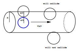
Consider two molecules in a system. The probability that they will collide increases with the effective “size” of each particle. However, the size measure that is relevant is the apparent cross-section area of each particle. For simplicity, suppose the particles are spherical, which is not a bad approximation for small molecules. If we are looking at a sphere, what we perceive as the size of the sphere is the cross section area of a great circle. Recall that each spherical particle has an associated “collision sphere” that just encloses two particles at closest contact, i.e., at the moment of a collision, and that this sphere is a radius \(d\), where \(d\) is the diameter of each spherical particle (see lecture 5). The cross-section of this collision sphere represents an effective cross section for each particle inside which a collision is imminent. The cross-section of the collision sphere is the area of a great circle, which is \(\pi d^2\). We denote this apparent cross section area \(\sigma\). Thus, for spherical particles \(A\) and \(B\) with diameters \(d_A\) and \(d_B\), the individual cross sections are
\[\sigma_A = \pi d_A^2, \: \: \: \sigma_B = \pi d_B^2 \label{11}\]
The collision cross section, \(\sigma_{AB}\) is determined by an effective diameter \(d_{AB}\) characteristic of both particles. The collision probability increases of both particles have large diameters and decreases if one of them has a smaller diameter than the other. Hence, a simple measure sensitive to this is the arithmetic average
\[d_{AB} = \dfrac{1}{2} \left( d_A + d_B \right) \label{12}\]
and the resulting collision cross section becomes
\[\begin{align} \sigma_{AB} &= \pi d_{AB}^2 \\ &= \pi \left( \dfrac{d_A + d_B}{2} \right)^2 \\ &= \dfrac{\pi}{4} \left( d_A^2 + 2d_A d_B + d_B^2 \right) \\ &= \dfrac{1}{4} \left( \sigma_A + 2 \sqrt{\sigma_A \sigma_B} + \sigma_B \right) \\ &= \dfrac{1}{2} \left[ \left( \dfrac{\sigma_A + \sigma_B}{2} \right) + \sqrt{\sigma_A \sigma_B} \right] \end{align} \label{13}\]
which, interestingly, is an average of the two types of averages of the two individual cross sections, the arithmetic and geometric averages!
Average collision Frequency
Consider a system of particles with individual cross sections \(\sigma\). A particle of cross section \(\sigma\) that moves a distance \(l\) in a time \(\Delta t\) will sweep out a cylindrical volume (ignoring the spherical caps) of volume \(\sigma l\) (Figure \(\PageIndex{1}\)). If the system has a number density \(\rho\), then the number of collisions that will occur is
\[N_{\text{coll}} = \rho \sigma l \label{14}\]
We define the average collision rate as \(N_{\text{coll}}/ \Delta t\), i.e.,
\[\gamma = \dfrac{N_{\text{coll}}}{\Delta t} = \dfrac{\rho \sigma l}{\Delta t} = \rho \sigma \langle | \textbf{v} | \rangle \label{15}\]
where \(\langle | \textbf{v} | \rangle\) is the average relative speed. If all of the particles are of the same type (say, type \(A\)), then performing the average over a Maxwell-Boltzmann speed distribution gives
\[\langle | \textbf{v} | \rangle = \sqrt{\dfrac{8 k_B T}{\pi \mu}} \label{16}\]
where \(\mu = m_A/2\) is the reduced mass. The average speed of a particle is
\[\langle | \textbf{v}_A | \rangle = \sqrt{\dfrac{8 k_B T}{\pi m_A}} \label{17}\]
so that
\[\langle | \textbf{v} | \rangle = \sqrt{2} \langle | \textbf{v}_A | \rangle \label{18}\]
Mean Free Path
The mean free path is defined as the distance a particle will travel, on average, before experiencing a collision event. This is defined as the product of the speed of a particle and the time between collisions. The former is \(\langle | \textbf{v} | \rangle/ \sqrt{2}\), while the latter is \(1/\gamma\). Hence, we have
\[\lambda = \dfrac{\langle | \textbf{v} |\rangle}{\sqrt{2} \rho \sigma \langle | \textbf{v} | \rangle} = \dfrac{1}{\sqrt{2} \rho \sigma} \label{19}\]
Random Walks
In any system, a particle undergoing frequent collisions will have the direction of its motion changed with each collision and will trace out a path that appears to be random. In fact, if we treat the process as statistical, then, we are, in fact, treating each collision event as a random event, and the particle will change its direction at random times in random ways! Such a path might appear as shown in Figure \(\PageIndex{2. Such a path is often referred to as a random walk path.
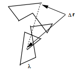
In order to analyze such paths, let us consider a random walk in one dimension. We’ll assume that the particle move a mean-free path length \(\lambda\) between collisions and that each collision changes the direction of the particles motion, which in one dimension, means that the particle moves either to the right or to the left after each event. This can be mapped onto a metaphoric “coin toss” that can come up heads “H” or tails “T”, with “H” causing motion to the right, and “T” causing motion to the left. Let there be \(N\) such coin tosses, let \(i\) be the number of times “H” comes up and \(j\) denote the number of times “T” comes up. Thus, the progress of the particle, which we define as net motion to the right, is given by \((i - j) \lambda\). Letting \(k = i - j\), this is just \(k \lambda\). Thus, we need to know what the probability is for obtaining a particular value of \(k\) in a very large number \(N\) of coin tosses. Denote this \(P(k)\).
In \(N\) coin tosses, the total number of possible sequences of “H” and “T” is \(2^N\). However, the number of ways we can obtain \(i\) heads and \)j\) tails, with \(i + j = N\) is a binomial coefficient \(N!/i!j!\). Now
\[j = N - i = N - (j + k) = N - j - k \label{20}\]
so that \(j = (N - k )/2\). Similarly,
\[i = N - j = N - (i - k) = N - i + k \label{21}\]
so that \(i = (N + k)/2\). Thus, the probability \(P(k)\) is
\[P(k) = \dfrac{N!}{2^N i! j!} = \dfrac{1}{2^N} \dfrac{N!}{\left(\dfrac{N + k}{2} \right) ! \left( \dfrac{N - k}{2} \right) !} \label{22}\]
We now take the logarithm of both sides:
\[\text{ln} \: P(k) = \: \text{ln} \: N! - \: \text{ln} \: 2^N - \: \text{ln} \: \left( \dfrac{N + k}{2} \right) ! - \: \text{ln} \: \left( \dfrac{N - k}{2} \right) ! \label{23}\]
and use Stirling’s approximation:
\[\text{ln} \: N! \approx N \: \text{ln} \: N - N \label{24}\]
and write \(\text{ln} \: P(k)\) as
\[\begin{align} \text{ln} \: P(k) &\approx N \: \text{ln} \: N - N - N \: \text{ln} \: 2 - \dfrac{1}{2} (N + k) \: \text{ln} \: \dfrac{1}{2} (N + k) + \dfrac{1}{2} (N + k) - \dfrac{1}{2} (N - k) \: \text{ln} \: \dfrac{1}{2} (N - k) + \dfrac{1}{2} (N - k) \\ &= N \: \text{ln} \: N - N \: \text{ln} \: 2 + \dfrac{1}{2} (N + k) \: \text{ln} \: \dfrac{1}{2} - \dfrac{1}{2} (N + k) \: \text{ln} \: (N + k) - \dfrac{1}{2} (N - k) \: \text{ln} \: \dfrac{1}{2} - \dfrac{1}{2} (N - k) \: \text{ln} \: (N - k) \\ &= N \: \text{ln} \: N - N \: \text{ln} \: 2 + \dfrac{1}{2} (N + k) \: \text{ln} \: 2 - \dfrac{1}{2} (N + k) \: \text{ln} \: (N + k) + \dfrac{1}{2} (N - k) \: \text{ln} \: 2 - \dfrac{1}{2} (N - k) \: \text{ln} \: (N - k) \\ &= N \: \text{ln} \: N - \dfrac{1}{2} \left[ (N + k) \: \text{ln} \: (N + k) + (N - k) \: \text{ln} \: (N - k) \right] \end{align} \label{25}\]
Now, write
\[\text{ln} \: (N + k) = \: \text{ln} \: N \left( 1 + \dfrac{k}{N} \right) = \: \text{ln} \: N + \: \text{ln} \: \left( 1 + \dfrac{k}{N} \right) \label{26}\]
and
\[\text{ln} \: (N - k) = \: \text{ln} \: N \left( 1 - \dfrac{k}{N} \right) = \: \text{ln} \: N + \: \text{ln} \: \left( 1 - \dfrac{k}{N} \right) \label{27}\]
We now use the expansions
\[\begin{align} \text{ln} \: \left( 1 + \dfrac{k}{N} \right) &= \left( \dfrac{k}{N} \right) - \dfrac{1}{2} \left( \dfrac{k}{N} \right)^2 + \cdots \\ \text{ln} \: \left( 1 - \dfrac{k}{N} \right) &= - \left( \dfrac{k}{N} \right) - \dfrac{1}{2} \left( \dfrac{k}{N} \right)^2 + \cdots \end{align} \label{28}\]
If we stop at the second-order term, then
\[\begin{align} \text{ln} \: P(k) &= N \: \text{ln} \: N - \dfrac{1}{2} (N + k) \left[ \: \text{ln} \: N + \left( \dfrac{k}{N} \right) - \dfrac{1}{2} \left( \dfrac{k}{N} \right)^2 \right] - \dfrac{1}{2} (N - k) \left[ \: \text{ln} \: N - \left( \dfrac{k}{N} \right) - \dfrac{1}{2} \left( \dfrac{k}{N} \right)^2 \right] \\ &= -\dfrac{1}{2} (N + k) \left[ \left( \dfrac{k}{N} \right) - \dfrac{1}{2} \left( \dfrac{k}{N} \right)^2 \right] + \dfrac{1}{2} (N - k) \left[ \left( \dfrac{k}{N} \right) + \dfrac{1}{2} \left( \dfrac{k}{N} \right)^2 \right] \\ &= \dfrac{1}{2} N \left( \dfrac{k}{N} \right)^2 - k \left( \dfrac{k}{N} \right) \\ & = \dfrac{k^2}{2N} - \dfrac{k^2}{N} = - \dfrac{k^2}{2N} \end{align} \label{29}\]
so that
\[P(k) = e^{-k^2/2N} \label{30}\]
Now, if we let \(x = k \lambda\) and \(L = \sqrt{N} \lambda\), and if we let \(x\) be a continuous random variable, then the corresponding probability distribution \(P(x)\) becomes
\[P(x) = \dfrac{1}{L \sqrt{2 \pi}} \: e^{-x^2/2L^2} = \dfrac{1}{\sqrt{2 \pi N \lambda^2}} \: e^{-x^2/2N \lambda^2} \label{31}\]
which is a simple Gaussian distribution. Now, \(N\) is the number of collisions, which is given by \(\gamma t\), so we can write the probability distribution for the particle to diffuse a distance \(x\) in time \(t\) as
\[P(x, t) = \dfrac{1}{\sqrt{2 \pi \gamma t \lambda^2}} \: e^{-x^2/2 \gamma t \lambda^2} \label{32}\]
Define \(D = \gamma \lambda^2/2\) as the diffusion constant, which has units of (length)\(^{\text{2}}\)/time. The distribution then becomes
\[P(x, t) = \dfrac{1}{\sqrt{4 \pi D t }} \: e^{-x^2/4D t} \label{33}\]
Note that this distribution satisfies the following equation:
\[\dfrac{\partial}{\partial t} P(x, t) = D \dfrac{\partial^2}{\partial x^2} P(x, t) \label{34}\]
which is called the diffusion equation. The diffusion equation is, in fact, more general than the Gaussian distribution in Equation \(\ref{33}\). It is capable of predicting the distribution in any one-dimensional geometry subject to any initial distribution \(P(x, 0)\) and any imposed boundary conditions.
In three dimensions, we consider the three spatial directions to be independent, hence, the probability distribution for a particle to diffuse to a location \(\textbf{r} = (x, y, z)\) is just a product of the three one-dimensional distributions:
\[\mathcal{P}(\textbf{r}) = P(x) \: P(y) \: P(z) = \dfrac{1}{(4 \pi D t) ^{3/2}} \: e^{-\left( x^2 + y^2 + z^2 \right)/4Dt} \label{35}\]
and if we are only interested in diffusion over a distance \(r\), we can introduce spherical coordinates, integrate over the angles, and we find that
\[P(r, t) = \dfrac{4 \pi}{(4 \pi D t)^{3/2}} \: E^{-r^2/4Dt} \label{36}\]