1.4: Treating interactions - Virial coefficients

The Isothermal-Isobaric Ensemble

The isothermal-isobaric ensemble is the closest mimic to the conditions under which most experiments are performed, namely under conditions of constant \(N\), \(P\), and \(T\). In order to fix the pressure and temperature, the system must allowed to exchange heat with its surrounds, and the surrounds must also act as a kind of isotropic “piston” on the system, allowing the system’s volume \(V\) to fluctuate in response to an applied pressure \(P\). If the volume fluctuates, then we can treat is as an additional mechanical variable in the system. If this is the case, then the energy \(E\) can change in response to the exchange of heat, while there is an additional energy term \(P \Delta V\), which when added to the energy change \(\Delta E\), gives the total energy change in response to both the piston and the heat exchange. This sum \(\Delta E + P \Delta V\) goes by the name “enthalpy” and is denoted \(\Delta H\):

\[\Delta H = \Delta E + P \Delta V \label{4.1} \]

The mechanical version of this simply replaced \(E\) by the mechanical energy \(\mathcal{E} (x)\), and we would integrate a Boltzmann distribution of \(\mathcal{E} (x) + PV\) over all coordinates, momenta, and volumes in order to produce a partition function:

\[\begin{align} \Delta (N, P, T) &= C_N \int \limits_0^\infty dV \int dx \: e^{-\beta (\mathcal{E} (x) + PV)} \\ &= \int \limits_0^\infty dV e^{-\beta PV}C_N \int dx \: e^{-\beta \mathcal{E} (x)} \\ &= \int \limits_0^\infty dV e^{-\beta PV} Q(N, V, T) \end{align} \label{4.2} \]

The last line of this shows that there is a very simple relation between the canonical partition function and that of the isothermal-isobaric ensemble. Once we know the canonical partition function, we just need to do one volume integral in order to determine the partition function of the isothermal-isobaric ensemble. The thermodynamic relations are also completely analogous to those of the canonical ensemble. Thus, the average enthalpy \(H\) is given by

\[H = -\frac{\partial}{\partial \beta} \: \text{ln} \: \Delta (N, P, T) \label{4.3} \]

and the constant-pressure heat capacity \(C_P\) becomes

\[C_P = k_B \beta^2 \frac{\partial^2}{\partial \beta^2} \: \text{ln} \: \Delta (N, P, T) \label{4.4} \]

The only real difference from the canonical ensemble is that we determine an average volume \(V\) from the pressure derivative of \(\Delta (N, P, T)\):

\[V = -k_BT \frac{\partial}{\partial P} \: \text{ln} \: \Delta (N, P, T) \label{4.5} \]

Treating Interactions: Virial Coefficients

We have seen that if we can determine a canonical partition function, then we can also easily compute the properties of a system at constant pressure by simply applying Equation 4.2. But how can we compute a canonical partition function for a system in which there are real interactions present?

One way is to use computer simulation techniques. If we run a molecular dynamics or Monte Carlo calculation, then, in addition to approximating the actual microscopic motion of a system, we are, in effect, using the simulation to “do 2 the many-dimensional integrals” over coordinates and momenta! Of course, the downside of this is that computer simulations can be time consuming, and they only allow us to examine one thermodynamic state point at a time. Each new state point is a new simulation. In addition, the computer will spit out reams of data, and we have, somehow, to make sense of it all. As the Hungarian-American physicist and Nobel laureate, Eugene Wigner once said, “It is nice to know that the computer understands the problem, but I would like to understand it too”. For this reason, analytical techniques can play an extremely valuable role, as they provide insights that cannot be easily gleaned from computer simulations.

Let us start, therefore, by considering a gas at low density and compute the canonical partition function for this system. We will assume that the density is sufficiently low that each particle interacts with just one other particle at a time (which would certainly not be the case in a liquid or solid). Because there interactions are pair-wise, we can assume that the potential energy is a sum of pair-wise terms:

\[U (\textbf{r}_1, \ldots, \textbf{r}_N) = \sum_{i=1}^{N-1} \sum_{j = i +1}^N u (|\textbf{r}_i - \textbf{r}_j|) \label{4.6} \]

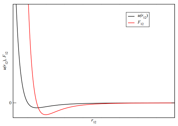
A typical plot of such a potential and the force it produces between two particles is shown in Figure 4.1. However, if each particle interacts with just one other particle at a time, then we can simplify the complicated sums above and write the potential as

\[U (\textbf{r}_1, \ldots, \textbf{r}_N) = u(|\textbf{r}_1 - \textbf{r}_2|) + u(|\textbf{r}_3 - \textbf{r}_4|) + \ldots u(|\textbf{r}_{N-1} - \textbf{r}_N|) \label{4.7} \]

provided that we recognize this as being just one possible way we can pair up the particles. If we account for all possible ways we can do this as a combinatorial factor in the counting of microstates, then we have all of the information we need to construct the partition function.

Figure 4.1: Typical potential energy and force curves for two particles in a real gas.

So let’s see how we can do this. Consider, first, the case of just four particles. In how many ways can we pair them up so that each particle interacts with just one other? There are, in fact, three possibilities. We have, for example, \((1, 2)(3, 4)\), but we also have \((1, 3)(2, 4)\), and \((1, 4)(2, 3)\). Note that the case \((1, 2)(3, 4)\) corresponds to what we have written in Equation 4.6. That is, for this pairing, we would write the potential as \(U (\textbf{r}_1, \textbf{r}_2, \textbf{r}_3, \textbf{r}_4) = u (|\textbf{r}_1 - \textbf{r}_2|) + u(|\textbf{r}_3 - \textbf{r}_4|)\). The three possibilities can be expressed as \(3 \cdot 1\).

Now suppose we had six particles. In how many ways can we pair these up. If you enumerate them all, you’ll find that there are 15 possibilities:

\[\begin{array}{c} (1, 2)(3, 4)(5, 6) \\ (1,2)(3, 5)(4, 6) \\ (1,2)(3,6)(4,5) \\ \\ (1,3)(2,4)(5,6) \\ (1,3)(2,5)(4,6) \\ (1,3)(2,6)(4,5) \\ \\ (1,4)(2,3)(5,6) \\ (1,4)(2,5)(3,6) \\ (1,4)(2,6)(3,5) \\ \\ (1,5)(2,3)(4,6) \\ (1,5)(2,4)(3,6) \\ (1,5)(2,6)(3,4) \\ \\ (1,6)(2,3)(4,5) \\ (1,6)(2,4)(3,5) \\ (1,6)(2,5)(3,4) \end{array} \nonumber \]

Note that \(15 = 5 \cdot 3 \cdot 1\). Thus, in general, if we have \(N\) particles, where \(N\) must be even so that we can pair them up, then the number of ways we can pair them up is \((N-1)(N-3)(N-5) \ldots = (N-1)!!\).

Recall that the canonical partition function is

\[Q(N, V, T) = C_N \int dx_{\textbf{p}} \: e^{-\beta \sum_{i=1}^N \textbf{p}_i^2/2m} \int dx_{\textbf{r}} \: e^{-\beta U (\textbf{r}_1, \ldots, \textbf{r}_N)} \label{4.8} \]

Let us denote by \(Z(N, V, T)\)

\[Z(N, V, T) = \int d \textbf{r}_1 \ldots d \textbf{r}_N \: e^{-\beta U (\textbf{r}_1, \ldots, \textbf{r}_N)} \label{4.9} \]

We will be interested in computing the equation of state for our system, which we obtain by computing the pressure from

\[P = k_BT \left( \frac{\partial \: \text{ln} \: Q}{\partial V} \right) \label{4.10} \]

However, \(Z(N, V, T)\) contains all of the volume dependence of \(Q\), so we really only need to worry about it, and the pressure would then be given by

\[P = k_BT \left( \frac{\partial \: \text{ln} \: Z}{\partial V} \right) \label{4.11} \]

In the limit that we can consider each particle as interacting with just one other particle at a time, for which there are \((N - 1)!!\) possible combinations, we can write \(Z\) as

\[\begin{align} Z(N, V, T) &= (N - 1)!! \int d \textbf{r}_1 \cdots d \textbf{r}_N \: e^{-\beta u (| \textbf{r}_1 - \textbf{r}_2|)} \: e^{-\beta u (| \textbf{r}_3 - \textbf{r}_4|)} \cdots \: e^{-\beta u (| \textbf{r}_{N - 1} - \textbf{r}_N|)} \\ &= (N - 1)!! \left[ \int d \textbf{r}_1 \: d \textbf{r}_2 \: e^{-\beta u (| \textbf{r}_1 - \textbf{r}_2|)} \right] \left[ \int d \textbf{r}_3 \: d \textbf{r}_4 \: e^{-\beta u (| \textbf{r}_3 - \textbf{r}_4|)} \right] \cdots \left[ \int d \textbf{r}_{N - 1} \: d \textbf{r}_N \: e^{-\beta u (| \textbf{r}_{N - 1} - \textbf{r}_N|)} \right] \end{align} \label{4.12} \]

All of the integrals in the brackets are exactly the same. Moreover, for \(N\) particles, there are \(N/2\) pairs we can make, so we can write the above expression as

\[Z(N, V, T) = (N-1)!! \left[ \int d \textbf{r}_1 \: d \textbf{r}_2 \: e^{-\beta u (| \textbf{r}_1 - \textbf{r}_2|)} \right]^{N/2} \label{4.13} \]

Next, let’s look at the prefactor of \((N-1)!!\). Recall that \(N! = N(N-1)(N-2) \cdots 1\). This is a product of \(N\) terms, and if \(N\) is \(N! \approx N^N e^{-N}\), which is known as Sterling’s approximation. Similarly for \((N-1)!! = (N-1)(N-3) \cdots 3 \cdot 1\), the leading term is \(N -1 \approx N\), and there are \(N/2\) terms in the product, so the approximation for a double factorial when \(N\) is large becomes \((N-1)!! \approx N^{N/2} e^{-N/2}\). Thus, we can write \(Z\) as

\[Z(N, V, T) \approx e^{-N/2} \left[ N \int d \textbf{r}_1 \: d \textbf{r}_2 \: e^{-\beta u (| \textbf{r}_1 - \textbf{r}_2|)} \right]^{N/2} \label{4.14} \]

In fact, the \(e^{-N/2}\) we can simply absorb into the \(C_N\) in the definition of \(Q\), as it is volume independent and will not affect anything our calculations. Thus, it is sufficient for us to consider simply

\[Z(N, V, T) \approx \left[ N \int d \textbf{r}_1 \: d \textbf{r}_2 \: e^{-\beta u (| \textbf{r}_1 - \textbf{r}_2|)} \right]^{N/2} \label{4.15} \]

In order to simplify the integral, let us change variables to

\[\begin{array}{cc}\textbf{R} = \frac{1}{2} (\textbf{r}_1 + \textbf{r}_2), & \textbf{r} = \textbf{r}_1 - \textbf{r}_2 \end{array} \label{4.16} \]

for which \(d \textbf{r}_1 d \textbf{r}_2 = d \textbf{R} d \textbf{r}\). Substituting this in, we obtain

\[Z(N, V, T) \approx \left[ N \int d \textbf{R} \: d \textbf{r} \: e^{-\beta u (| \textbf{r}|)} \right]^{N/2} \label{4.17} \]

Since the integrand does not depend on \(\textbf{R}\), we can easily integrate over \(\textbf{R}\):

\[\int d \textbf{R} = \int \limits_0^a dX \int \limits_0^a dY \int \limits_0^a dZ = a^3 = V \label{4.18} \]

Then

\[Z(N, V, T) = V^{N/2} \left[ N \int d \textbf{r} \: e^{-\beta u (| \textbf{r}|)} \right]^{N/2} \label{4.19} \]

The remaining integral still has an implied volume dependence in the sense that

\[\int d \textbf{r} \: e^{-\beta u (| \textbf{r}|)} = \int \limits_0^a dx \int \limits_0^a dy \int \limits_0^a dz \: e^{-\beta u (| \textbf{r}|)} \nonumber \]

In order to make this volume dependence easier to work with, we go into a set of scaled coordinates

\[\textbf{s} = \frac{\textbf{r}}{a} = \frac{\textbf{r}}{V^{1/3}} = V^{-1/3} \textbf{r} \label{4.20} \]

The components of \(\textbf{s}\) all lie in the interval \([0, 1]: s_x \in [0, 1], s_y \in [0, 1], s_z \in [0, 1]\). Moreover, \(d \textbf{r} = dx \: dy \: dz = a^3ds_x \: ds_y \: ds_z = Vd \textbf{s}\). Putting this into the partition function, we have

\[\begin{align} Z(N, V, T) &= V^{N/2} \left[ NV \int d \textbf{s} \: e^{-\beta u (| v^{1/3} \textbf{s}|)} \right]^{N/2} \\ &= V^N \left[ N \int d \textbf{s} \: e^{-\beta u (|V^{1/3} \textbf{s}|)} \right]^{N/2} \end{align} \label{4.21} \]

This is now an expression we can differentiate with respect to \(V\) to obtain the pressure. Using Equation 4.11, we find

\[\begin{align} P &= k_B T \frac{\partial}{\partial V} \left\{ \text{ln} \: V^N + \text{ln} \left[ N \int d \textbf{s} \: e^{-\beta u (|V^{1/3} \textbf{s}|)} \right]^{N/2} \right\} \\ &= k_B T \frac{\partial}{\partial V} \left\{ N \: \text{ln} \: V + \frac{N}{2} \: \text{ln} \left[ N \int d \textbf{s} \: e^{-\beta u (|V^{1/3} \textbf{s}|)} \right] \right\} \\ &= \frac{Nk_BT}{V} + k_BT \frac{\partial}{\partial V} \left\{ \frac{N}{2} \: \text{ln} \left[ N \int d \textbf{s} \: e^{-\beta u (|V^{1/3} \textbf{s}|)} k \right] \right\} \end{align} \label{4.22} \]

Let

\[I (V) = \int d \textbf{s} \: e^{-\beta u (|V^{1/3} \textbf{s}|)} \label{4.23} \]

If we assume that the interaction is a small perturbation to ideal-gas behavior, then we can take \(I(V)\) to be a small quantity. In fact, we will see below that because \(dI/dV \sim 1/V^2\), \(I(V) \sim 1/V\), and since \(1/V \sim 1/N\), \(I(V) \sim 1/N\). In this case, \(NI(V) \sim 1\), and we can use the approximation \(\text{ln} \: (1 + x) \approx x\) to write

\[\text{ln} \: NI(V) = \: \text{ln} \: (1 + NI(V) - 1) \approx (NI(V) - 1) \label{4.24} \]

so that

\[P = \frac{Nk_BT}{V} + \frac{Nk_BT}{2} \frac{\partial}{\partial V} (NI(V) - 1) = \frac{Nk_BT}{V} + \frac{N^2k_BT}{2} \frac{\partial I}{\partial V} \label{4.25} \]

Let’s now look at the volume derivative of \(I(V)\). Applying the chain rule, we have

\[\frac{\partial I}{\partial V} = -\beta \int d \textbf{s} \frac{\partial u}{\partial (V^{1/3} \textbf{s})} \cdot \textbf{s} \frac{1}{3} V^{-2/3} e^{-\beta u (|V^{1/3} \textbf{s}|)} \label{4.26} \]

Now that we’ve taken the volume derivative, we can go back to unscaled coordinates via \(\textbf{s} = V^{-1/3} \textbf{r}\). Remember \(d \textbf{s} = (1/V) d \textbf{r}\). If we do this, then the integral looks much less ugly:

\[\frac{\partial I}{\partial V} = -\frac{\beta}{3V^2} \int d \textbf{r} \frac{\partial u}{\partial \textbf{r}} \cdot \textbf{r} \: e^{-\beta u (| \textbf{r}|)} \label{4.27} \]

The term appearing in the integrand

\[\textbf{r} \frac{\partial u}{\partial \textbf{r}} \nonumber \]

comes up frequently in classical mechanics and is called the virial. Recognizing that \(u (| \textbf{r}|)\) is a function of \(r = |\textbf{r}|\), which is just the length of the vector \(\textbf{r}\), it follows that

\[\begin{align} \frac{\partial u}{\partial \textbf{r}} &= \frac{du}{dr} \frac{\partial r}{\partial \textbf{r}} \\ &= \frac{du}{dr} \frac{\textbf{r}}{r} \end{align} \label{4.28} \]

so that

\[\textbf{r} \cdot \frac{\partial u}{\partial \textbf{r}} = \frac{\partial u}{\partial r} \textbf{r} \cdot \frac{\textbf{r}}{r} = r \frac{du}{dr} \label{4.29} \]

Thus,

\[\frac{\partial I}{\partial V} = -\frac{\beta}{3V^2} \int d \textbf{r} \: r \frac{du}{dr} e^{-\beta u (r)} \label{4.30} \]

Now transform to spherical polar coordinates in \(\textbf{r}\), which gives

\[\frac{\partial I}{\partial V} = -\frac{\beta}{3V^2} \int \limits_0^{2 \pi} d \phi \int \limits_0^\pi d \theta \sin \theta \int \limits_0^\infty dr \: r^3 \frac{du}{dr} e^{-\beta u (r)} \label{4.31} \]

Note that we have made the approximation that the \(r\) integral can be taken from \(0\) to \(\infty\). Strictly speaking, this is wrong because this integral should be limited by the maximum \(r\) allowed by the containing volume. However, as Figure 4.1 indicates, \(u'(r) = \partial u/ \partial r\) vanishes very quickly as \(r\) increases, so that the integrand in the above integral goes to \(0\) long before we hit the boundary of the box. Given that, extending the integral out to \(\infty\) just adds a lot of zero to the integral, which will not change the answer!

Integrating over the angles, we obtain

\[\frac{\partial I}{\partial V} = -\frac{4 \pi \beta}{3V^2} \int \limits_0^\infty dr \: r^3 \frac{du}{dr} e^{-\beta u (r)} \label{4.32} \]

We now simplify this expression by the integral as

\[\frac{\partial I}{\partial V} = \frac{4 \pi \beta}{3V^2} \frac{1}{\beta} \int \limits_0^\infty dr \: r^3 \frac{d}{dr} e^{-\beta u (r)} \label{4.33} \]

which we can integrate by parts to give

\[\frac{\partial I}{\partial V} = \frac{4 \pi}{3V^2} \left[ r^3 \left. e^{-\beta u (r)} \right|_0^\infty - \int \limits_0^\infty dr \left( \frac{d}{dr} r^3 \right) e^{-\beta u (r)} \right] \label{4.34} \]

Unfortunately, when we try to evaluate the first term, we find that it is \(\infty\) at \(r = \infty\). Even if we admit that this is a consequence of our approximation that \(r\) can be integrated out to \(\infty\), it does not really matter because this term would simply increase with increasing system size, i.e., increasing volume, which is unphysical, as the pressure cannot behave this way – pressure is an intensive quantity. Fortunately, there is a trick that can save us. Recognizing that \(u(r) \rightarrow 0\) as \(r \rightarrow \infty\), \(exp(-\beta u (r)) \rightarrow 1\) as \(r \rightarrow \infty\). Hence, let us back up and just subtract this one from the exponential where we introduce the derivative. That is, if we write

\[\frac{\partial I}{\partial V} = \frac{4 \pi \beta}{3V^2} \frac{1}{\beta} \int \limits_0^\infty dr \: r^3 \frac{d}{dr} e^{-\beta u (r)} = \frac{4 \pi \beta}{3V^2} \frac{1}{\beta} \int \limits_0^\infty dr \: r^3 \frac{d}{dr} (e^{-\beta u (r)} - 1) \label{4.35} \]

we do not change anything since the derivative of \(1\) with respect to \(r\) is \(0\) anyway. We can now integrate this by parts to give

\[\frac{\partial I}{\partial V} = \frac{4 \pi}{3V^2} \left[ r^3 \left( \left. e^{-\beta u (r)} - 1 \right) \right|_0^\infty - \int \limits_0^\infty dr \left( \frac{d}{dr} \: r^3 \right) \left( e^{-\beta u (r)} - 1 \right) \right] \label{4.36} \]

Now the first term vanishes both at \(r = 0\) and at \(r = \infty\), and we are left with

\[\frac{\partial I}{\partial V} = -\frac{4 \pi}{V^2} \int \limits_0^\infty dr \: r^2 \left( e^{-\beta u (r)} - 1 \right) \label{4.37} \]

and the pressure becomes

\[P = \frac{Nk_BT}{V} - \frac{N^2 k_BT}{V^2} \: 2 \pi \int \limits_0^\infty dr \: r^2 \left( e^{-\beta u (r)} - 1 \right) \label{4.38} \]

Using the fact that \(R = N_0 k_B\), and introducing the density \(\rho = n/V\), we finally obtain

\[\begin{align} P &= \rho RT + \rho^2 RT \left[ -2 \pi N_0 \int \limits_0^\infty dr \: r^2 \left( e^{-\beta u (r)} - 1 \right) \right] \\ \frac{P}{\rho RT} &= 1 + \rho \left[ -2 \pi N_0 \int \limits_0^\infty dr \: r^2 \left( e^{-\beta u (r)} - 1 \right) \right] \end{align} \label{4.39} \]

The term in brackets is denoted \(B_2(T)\):

\[B_2(T) = -2 \pi N_0 \int \limits_0^\infty dr \: r^2 \left( e^{-\beta u (r)} - 1 \right) \label{4.40} \]

and is called a virial coefficient, as it arises from the classical mechanical virial mentioned above.

More realistic treatments of non-ideal gases generate an equation of state in the form of a power series in the density in which all of the coefficients are functions of temperature. This can be expressed as

\[\frac{P}{\rho RT} = 1 + \sum_{k = 1}^\infty B_{k+1} (T) \rho^k \label{4.41} \]

This equation of state is called the virial equation of state. The coefficients \(B_{k+1}(T)\)are called virial coefficients. In the low density limit, the most important term in this power series is the \(k = 1\) or linear term, which gives the approximate equation of state

\[\frac{P}{\rho RT} \approx 1 + B_2(T) \rho \label{4.42} \]

where the dominant coefficient \(B_2(T)\) is called the second virial coefficient. These can be measured experimentally. The following plot shows the second virial coefficient for several gases. Although it is difficult to see, these curves pass

Figure 4.2: Experimental second virial coefficient plots for several real gases.

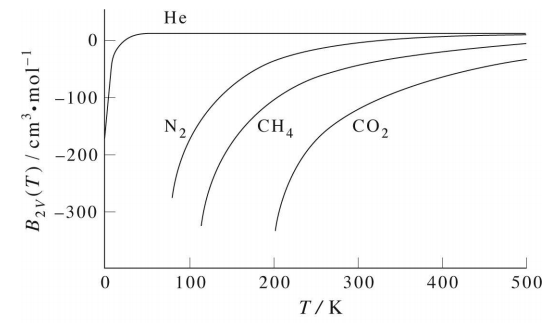
through a shallow maximum that is not captured by the van der Waals equation. Thus, the van der Waals equation is only in qualitative agreement with these but is not fully quantitative.

Let us look at some simple examples of \(B_2(T)\) calculations.

1. Hard-sphere potential:

\[u(r) = \begin{cases} \infty & r \leq \sigma \\ 0 & r > \sigma \end{cases} \label{4.43} \]

For this potential, the calculation of \(B_2(T)\) proceeds as follows:

\[\begin{align} B_2(T) &= -2 \pi N_0 \left[ \int \limits_0^\sigma \left( e^{-\beta \cdot \infty} - 1 \right) r^2 dr + \int \limits_\sigma^\infty \left( e^{-\beta \cdot 0} - 1 \right) r^2 dr \right] \\ &= -2 \pi N_0 \left[ \int \limits_0^\sigma (0 -1) \: r^2 dr + \int \limits_\sigma^\infty (1 - 1) \: r^2 dr \right] \\ &= 2 \pi N_0 \int \limits_0^\sigma r^2 dr \\ &= \frac{2}{3} \pi \sigma^3 N_0 \end{align} \label{4.44} \]

which is also the parameter \(b\) in the van der Waals equation. In this case, there is no temperature dependence in the result for \(B_2(T)\).

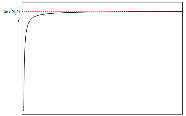
2. Square-well potential plus hard-sphere potential: In this case, the potential takes the form

\[u(r) = \begin{cases} \infty & r \leq \sigma \\ -\epsilon & \sigma \leq r \leq \lambda \sigma \\ 0 & r > \lambda \sigma \end{cases} \label{4.45} \]

In this case, the hard-sphere potential is supplemented by a short-range constant attractive potential that has a “square-well” shape. The parameter \(\lambda > 1\) determines the range of the square well. For this example, the calculation of \(B_2(T)\) proceeds as follows:

\[\begin{align} B_2(T) &= -2 \pi N_0 \left[ \int \limits_0^\sigma \left( e^{-\beta \cdot \infty} - 1 \right) r^2 dr + \int \limits_\sigma^{\lambda \sigma} \left( e^{\beta \epsilon} - 1 \right) r^2 dr + \int \limits_{\lambda \sigma}^\infty \left( e^{-\beta \cdot 0} - 1 \right) r^2 dr \right] \\ &= -2 \pi N_0 \left[ - \int \limits_0^\sigma r^2 dr + \left( e^{\beta \epsilon} - 1 \right) \int \limits_{\lambda \sigma}^\infty r^2 dr \right] \\ &= -2 \pi N_0 \left[ - \frac{\sigma^3}{3} + \left( e^{\beta \epsilon} - 1 \right) \left. \frac{r^3}{3} \right|_\sigma^{\lambda \sigma} \right] \\ &= -2 \pi N_0 \left[ -\frac{\sigma^3}{3} + \left( e^{\beta \epsilon} - 1 \right) \frac{1}{3} \left( \lambda^3 \sigma^3 - \sigma^3 \right) \right] \\ &= \frac{2 \pi N_0 \sigma^3}{3} \left[ 1 - \left( e^{\beta \epsilon} - 1 \right) \left( \lambda^3 - 1 \right) \right] \end{align} \label{4.46} \]

A plot of this second virial coefficient is given in the figure below.

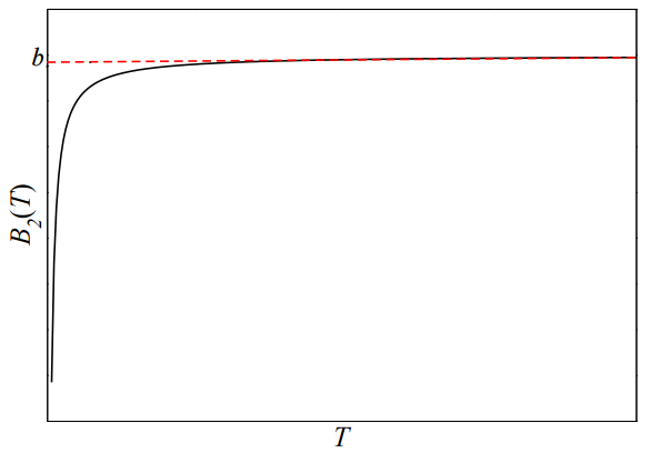
3. Hard-sphere plus \(-C_6/r^6\) potential: For this example, the potential is

\[u(r) = \begin{cases} \infty & r \leq \sigma \\ - \frac{C_6}{r^6} & r > \sigma \end{cases} \label{4.47} \]

This is a particular realization of a potential that leads to the van der Waals equation of state. The \(-C_6/r^6\) attractive part of the potential comes directly from a full quantum mechanical treatment of the electron distribution around each atom in an interacting pair. Such an attractive potential attempts to model London dispersion or van der Waals forces. For this example, the calculation of \(B_2(T)\) proceeds as follows:

\[\begin{align} B_2(T) &= -2 \pi N_0 \left[ \int \limits_0^\sigma \left( e^{-\beta \cdot \infty} - 1 \right) r^2 dr + \int \limits_\sigma^\infty \left( e^{\beta C_6/r^6} -1 \right) r^2 dr \right] \\ &= -2 \pi N_0 \left[ -\frac{\sigma^3}{3} + \int \limits_\sigma^\infty \left( e^{\beta C_6/r^6} - 1 \right) r^2 dr \right] \end{align} \label{4.48} \]

Figure 4.3: Second virial coefficient for the hard-sphere plus square-well potential.

The remaining integral cannot be evaluated in closed form, but let us suppose that \(\beta C_6/r^6 \ll 1\) for all values of \(r\) considered, i.e., \(\sigma \leq r < \infty\). Then, we can expand the exponential using the power series \(e^x \approx 1 + x + x^2/2! + \cdots\). If we retain just the first two terms, then we have the approximation

\[e^{\beta C_6/r^6} - 1 \approx 1 + \frac{\beta C_6}{r^6} - 1 = \frac{\beta C_6}{r^6} \label{4.49} \]

With this approximation, the calculation of \(B_2(T)\) can proceed as follows:

\[\begin{align} B_2(T) &\approx -2 \pi N_0 \left[ -\frac{\sigma^3}{3} + \beta C_6 \int \limits_\sigma^\infty \frac{1}{r^6} \: r^2 dr \right] \\ &= -2 \pi N_0 \left[ -\frac{\sigma^3}{3} + \beta C_6 \int \limits_\sigma^\infty \frac{1}{r^4} dr \right] \\ &= -2 \pi N_0 \left[ -\frac{\sigma^3}{3} + \beta C_6 \left( \left. -\frac{1}{3r^3} \right|_\sigma^\infty \right) \right] \\ &= -2 \pi N_0 \left[ -\frac{\sigma^3}{3} + \frac{\beta C_6}{3 \sigma^3} \right] \\ &= \frac{2 \pi N_0 \sigma^3}{3} \left[ 1 - \frac{C_6}{3k_BT \sigma^6} \right] \end{align} \label{4.50} \]

A plot of this function will follow the curve presented in the figure below.

Figure 4.4: Second virial coefficient for the hard-sphere plus \(-C_6/r^6\) potential.

However, in this example, we can improve the approximation by retaining more terms of the exponential we expanded above. In fact, let us see what happens if we retain all of the terms in the power series. That is, we will use the fact that \(e^x\) can be represented exactly as

\[e^x = \sum_{k = 0}^\infty \frac{x^k}{k!} = 1 + \sum_{k = 1}^\infty \frac{x^k}{k!} \label{4.51} \]

so that

\[\begin{align} e^{\beta C_6/r^6} - 1 &= \sum_{k = 1}^\infty \frac{1}{k!} \left( \frac{\beta C_6}{r^6} \right)^k \\ &= 1 + \sum_{k = 1}^\infty \frac{\beta^k C_6^k}{k!} \frac{1}{r^{6k}} \end{align} \label{4.52} \]

With the expansion, the calculation of \(B_2(T)\) proceeds as follows:

\[\begin{align} B_2(T) &= -2 \pi N_0 \left[ -\frac{\sigma^3}{3} + \sum_{k = 1}^\infty \frac{\beta^k C_6^k}{k!} \int \limits_\sigma^\infty \frac{1}{r^{6k}} \: r^2 dr \right] \\ &= -2 \pi N_0 \left[ -\frac{\sigma^3}{3} + \sum_{k = 1}^\infty \frac{\beta^k C_6^k}{k!} \int \limits_\sigma^\infty \frac{1}{r^{6k - 2}} dr \right] \\ &= -2 \pi N_0 \left[ -\frac{\sigma^3}{3} + \sum_{k = 1}^\infty \frac{\beta^k C_6^k}{k!} \frac{1}{\left( 6k - 1 \right) \sigma^{6k - 1}} \right] \\ &= \frac{2 \pi N_0 \sigma^3}{3} \left[ 1 - 3 \sum_{k = 1}^\infty \frac{\left( \beta C_6 \right)^k}{k!} \frac{1}{ \left( 6k - 1 \right) \sigma^{6k + 2}} \right] \end{align} \label{4.53} \]

The final result represents an exact expression for \(B_2(T)\) for this particular model of \(u(r)\). How does it improve on the result obtained above retaining just two terms in the expansion of the exponential? Let us plot the final result as a function of temperature in the following way: Unfortunately, we cannot resum the final expression into a nice closed form, but we can evaluate the sum numerically on a computer. However, on a computer, we cannot sum an infinite number of terms. Rather, we replace the upper limit of \(\infty\) with a maximum number of terms \(K_{\text{max}}\) and then just increase \(K_{\text{max}}\) until the result converges. So, let’s do that for several values of \(K_{\text{max}}\) and see how the curve changes as we increase \(K_{\text{max}}\). This will show us how the result converges with \(K_{\text{max}}\). The result is shown in the figure below. We see from the figure that the sum converges very rapidly with \(K_{\text{max}}\)

Figure 4.5: Second virial coefficient for the potential in Equation 4.47.

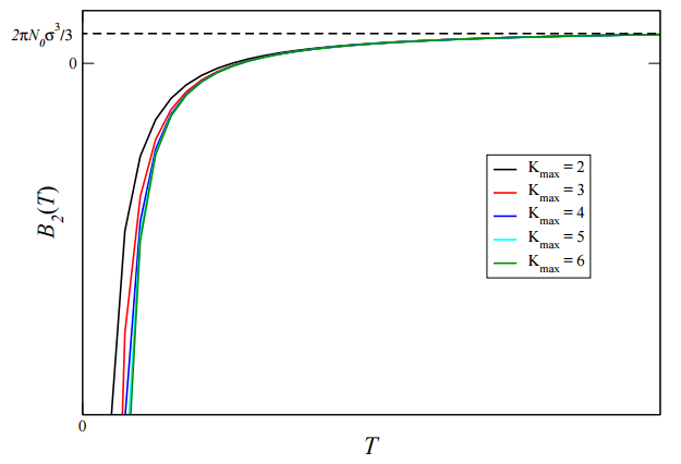
and only requires a few terms. Not unexpectedly, the most significant deviations from \(K_{\text{max}} = 2\) occur in the low-temperature part of the curves.

4. Perhaps the most realistic representation of the potential \(u(r)\) shown in Figure 2.2 is the so-called Lennard-Jones potential, for which

\[u(r) = 4 \epsilon \left[ \left( \frac{\sigma}{r} \right)^{12} - \left( \frac{\sigma}{r} \right)^6 \right] \label{4.54} \]

A plot of this potential very closely resembles that shown in Figure 2.2. In particular, there is a well-defined minimum, which we can compute by taking the derivative of \(u(r)\), setting it to \(0\), and solving for \(r\) at that point:

\[\begin{align} U'(r) = -4 \epsilon \left[ \frac{12 \sigma^{12}}{r^{13}} - \frac{6 \sigma^6}{r^7} \right] &= 0 \\ \frac{12 \sigma^{12}}{r^{13}} &= \frac{6 \sigma^6}{r^7} \\ \frac{2 \sigma^6}{r^{13}} &= \frac{1}{r^7} \\ 2 \sigma^6 &= r^6 \\ r &= 2^{1/6} \sigma \equiv r_m \end{align} \label{4.55} \]

where \(r_m\) denotes the location of the minimum. The value of the Lennard-Jones potential at that point is

\[\begin{align} u(r_m) = u \left( 2^{1/6} \sigma \right) &= 4 \epsilon \left[ \left( \frac{\sigma}{2^{1/6} \sigma} \right)^{12} \left( \frac{\sigma}{2^{1/6} \sigma} \right)^6 \right] \\ &= 4 \epsilon \left[ \frac{1}{2^2} - \frac{1}{2} \right] \\ &= -4 \epsilon \cdot \frac{1}{4} \\ &= - \epsilon \end{align} \label{4.56} \]

Thus, the parameter \(\epsilon\) measures the depth of the minimum at \(r = r_m\). In addition, \(u (\sigma)\), and for \(r < \sigma\), the potential exhibits a very steep increase, very much like the hard-sphere potential. Hence, \(\sigma\) is a measure of the van der Waals radius of each particle.

The calculation of the second virial coefficient can now be set up as

\[B_2(T) = -2 \pi N_0 \int \limits_0^\infty \left\{ exp \left( -4 \beta \epsilon \left[ \left( \frac{\sigma}{r} \right)^{12} - \left( \frac{\sigma}{r} \right)^6 \right] - 1 \right) \right\} r^2 dr \label{4.57} \]

Let us make a change of variables from \(r\) to

\[x = \frac{r}{\sigma} \nonumber \]

so that \(dr = \sigma dx\). Let us also define \(\beta^* = \beta \epsilon\). With this change, the integral for \(B_2(T)\) becomes

\[B_2(T) = -2 \pi \sigma^3 N_0 \int \limits_0^\infty \left[ e^{-4 \beta^* \left( x^{-12} - x^{-6} \right) } - 1 \right] x^2 dx \label{4.58} \]

Again, this integral cannot be evaluated analytically in closed form. We could expand the exponential in an infinite series as we did in the previous example. However, if we were to do this, the evaluation of the various terms in the integral would be considerably more complicated than in the previous example, as we would need to evaluated increasingly higher powers of a binomial form \((x^{-12} - x^{-6})^k\). Instead, since this is just a one-dimensional integral, we can evaluate it numerically using a method such as Simpson’s rule. Recall that Simpson’s rule for the integral of a function \(f(x)\) using a set of \(n\) evenly spaced values for \(x \: (x_0, x_1, \ldots, x_n)\) is just

\[\int \limits_a^b f(x)dx \approx \frac{h}{3} \left[ f(x_0) + 4f(x_1) + 2f(x_2) + 4f(x_3) + 2f(x_4) + \cdots + 2f(x_{n-2}) + 4f(x_{n-1}) + f(x_n) \right] \label{4.59} \]

where \(h = (b - a)/n\), and the points \(x_0, \ldots, x_n\) are given by \(x_j = a + jh, j = 0, \ldots, n\).

Applying this to the integral in Equation 4.58, the resulting curve for \(B_2(T)\) as a function of \(T\) appears as in the figure below: In this figure, \(k_BT^* = 1/\beta^*\), and

Figure 4.6: Second virial coefficient for the Lennard-Jones potential evaluated using numerical integration. Experimental points are also plotted. Because of the use of “reduced” units, data for all gases land on a single master curve, as an example of the law of corresponding states.

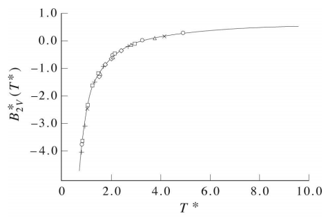
\[B_2^*(T) = \frac{B_2(T)}{2 \pi \sigma^3 N_0/3} \nonumber \]

Unfortunately, the curve in the book does not carry the curve out to high enough temperature to see the maximum. However, on page 233 of the book Statistical Mechanics by Donald A. McQuarrie, a more complete curve for the Lennard-Jones potential is shown, and in this curve the temperature axis is sufficiently long to see the maximum. This book is available on Google Books.