
8: The Quantum Hydrogen Atom
- Page ID
- 16974

\( \newcommand{\vecs}[1]{\overset { \scriptstyle \rightharpoonup} {\mathbf{#1}} } \)
\( \newcommand{\vecd}[1]{\overset{-\!-\!\rightharpoonup}{\vphantom{a}\smash {#1}}} \)
\( \newcommand{\id}{\mathrm{id}}\) \( \newcommand{\Span}{\mathrm{span}}\)
( \newcommand{\kernel}{\mathrm{null}\,}\) \( \newcommand{\range}{\mathrm{range}\,}\)
\( \newcommand{\RealPart}{\mathrm{Re}}\) \( \newcommand{\ImaginaryPart}{\mathrm{Im}}\)
\( \newcommand{\Argument}{\mathrm{Arg}}\) \( \newcommand{\norm}[1]{\| #1 \|}\)
\( \newcommand{\inner}[2]{\langle #1, #2 \rangle}\)
\( \newcommand{\Span}{\mathrm{span}}\)
\( \newcommand{\id}{\mathrm{id}}\)
\( \newcommand{\Span}{\mathrm{span}}\)
\( \newcommand{\kernel}{\mathrm{null}\,}\)
\( \newcommand{\range}{\mathrm{range}\,}\)
\( \newcommand{\RealPart}{\mathrm{Re}}\)
\( \newcommand{\ImaginaryPart}{\mathrm{Im}}\)
\( \newcommand{\Argument}{\mathrm{Arg}}\)
\( \newcommand{\norm}[1]{\| #1 \|}\)
\( \newcommand{\inner}[2]{\langle #1, #2 \rangle}\)
\( \newcommand{\Span}{\mathrm{span}}\) \( \newcommand{\AA}{\unicode[.8,0]{x212B}}\)
\( \newcommand{\vectorA}[1]{\vec{#1}} % arrow\)
\( \newcommand{\vectorAt}[1]{\vec{\text{#1}}} % arrow\)
\( \newcommand{\vectorB}[1]{\overset { \scriptstyle \rightharpoonup} {\mathbf{#1}} } \)
\( \newcommand{\vectorC}[1]{\textbf{#1}} \)
\( \newcommand{\vectorD}[1]{\overrightarrow{#1}} \)
\( \newcommand{\vectorDt}[1]{\overrightarrow{\text{#1}}} \)
\( \newcommand{\vectE}[1]{\overset{-\!-\!\rightharpoonup}{\vphantom{a}\smash{\mathbf {#1}}}} \)
\( \newcommand{\vecs}[1]{\overset { \scriptstyle \rightharpoonup} {\mathbf{#1}} } \)
\( \newcommand{\vecd}[1]{\overset{-\!-\!\rightharpoonup}{\vphantom{a}\smash {#1}}} \)
\(\newcommand{\avec}{\mathbf a}\) \(\newcommand{\bvec}{\mathbf b}\) \(\newcommand{\cvec}{\mathbf c}\) \(\newcommand{\dvec}{\mathbf d}\) \(\newcommand{\dtil}{\widetilde{\mathbf d}}\) \(\newcommand{\evec}{\mathbf e}\) \(\newcommand{\fvec}{\mathbf f}\) \(\newcommand{\nvec}{\mathbf n}\) \(\newcommand{\pvec}{\mathbf p}\) \(\newcommand{\qvec}{\mathbf q}\) \(\newcommand{\svec}{\mathbf s}\) \(\newcommand{\tvec}{\mathbf t}\) \(\newcommand{\uvec}{\mathbf u}\) \(\newcommand{\vvec}{\mathbf v}\) \(\newcommand{\wvec}{\mathbf w}\) \(\newcommand{\xvec}{\mathbf x}\) \(\newcommand{\yvec}{\mathbf y}\) \(\newcommand{\zvec}{\mathbf z}\) \(\newcommand{\rvec}{\mathbf r}\) \(\newcommand{\mvec}{\mathbf m}\) \(\newcommand{\zerovec}{\mathbf 0}\) \(\newcommand{\onevec}{\mathbf 1}\) \(\newcommand{\real}{\mathbb R}\) \(\newcommand{\twovec}[2]{\left[\begin{array}{r}#1 \\ #2 \end{array}\right]}\) \(\newcommand{\ctwovec}[2]{\left[\begin{array}{c}#1 \\ #2 \end{array}\right]}\) \(\newcommand{\threevec}[3]{\left[\begin{array}{r}#1 \\ #2 \\ #3 \end{array}\right]}\) \(\newcommand{\cthreevec}[3]{\left[\begin{array}{c}#1 \\ #2 \\ #3 \end{array}\right]}\) \(\newcommand{\fourvec}[4]{\left[\begin{array}{r}#1 \\ #2 \\ #3 \\ #4 \end{array}\right]}\) \(\newcommand{\cfourvec}[4]{\left[\begin{array}{c}#1 \\ #2 \\ #3 \\ #4 \end{array}\right]}\) \(\newcommand{\fivevec}[5]{\left[\begin{array}{r}#1 \\ #2 \\ #3 \\ #4 \\ #5 \\ \end{array}\right]}\) \(\newcommand{\cfivevec}[5]{\left[\begin{array}{c}#1 \\ #2 \\ #3 \\ #4 \\ #5 \\ \end{array}\right]}\) \(\newcommand{\mattwo}[4]{\left[\begin{array}{rr}#1 \amp #2 \\ #3 \amp #4 \\ \end{array}\right]}\) \(\newcommand{\laspan}[1]{\text{Span}\{#1\}}\) \(\newcommand{\bcal}{\cal B}\) \(\newcommand{\ccal}{\cal C}\) \(\newcommand{\scal}{\cal S}\) \(\newcommand{\wcal}{\cal W}\) \(\newcommand{\ecal}{\cal E}\) \(\newcommand{\coords}[2]{\left\{#1\right\}_{#2}}\) \(\newcommand{\gray}[1]{\color{gray}{#1}}\) \(\newcommand{\lgray}[1]{\color{lightgray}{#1}}\) \(\newcommand{\rank}{\operatorname{rank}}\) \(\newcommand{\row}{\text{Row}}\) \(\newcommand{\col}{\text{Col}}\) \(\renewcommand{\row}{\text{Row}}\) \(\newcommand{\nul}{\text{Nul}}\) \(\newcommand{\var}{\text{Var}}\) \(\newcommand{\corr}{\text{corr}}\) \(\newcommand{\len}[1]{\left|#1\right|}\) \(\newcommand{\bbar}{\overline{\bvec}}\) \(\newcommand{\bhat}{\widehat{\bvec}}\) \(\newcommand{\bperp}{\bvec^\perp}\) \(\newcommand{\xhat}{\widehat{\xvec}}\) \(\newcommand{\vhat}{\widehat{\vvec}}\) \(\newcommand{\uhat}{\widehat{\uvec}}\) \(\newcommand{\what}{\widehat{\wvec}}\) \(\newcommand{\Sighat}{\widehat{\Sigma}}\) \(\newcommand{\lt}{<}\) \(\newcommand{\gt}{>}\) \(\newcommand{\amp}{&}\) \(\definecolor{fillinmathshade}{gray}{0.9}\)Now that we have introduced the basic concepts of quantum mechanics, we can start to apply these concepts to build up matter, starting from its most elementary constituents, namely atoms, up to molecules, supramolecular complexes (complexes built from weak interactions such as hydrogen bonds and van der Waals interactions), networks, and bulk condensed phases, including liquids, glasses, solids,... As explore the structure of matter, itself, we should stand back and wonder at how the mathematically elegant, yet somehow not quite tangible, structure of quantum theory is able to describe so accurately all phases of matter and types of substances, ranging from metallic and semiconducting crystals to biological macromolecules, to morphologically complex polymeric materials.
We begin with the simplest system, the hydrogen atom (and hydrogen-like single-electron cations), which is the only atomic system (thus far) for which the Schrödinger equation can be solved exactly for the energy levels and wave functions. To this end, we consider a nucleus of charge \(+Ze\) at the origin and a single electron a distance \(r\) away from it. If we just naïvely start by writing the (total) classical energy
\[\underbrace{\dfrac{p_{x}^{2}}{2m}+\dfrac{p_{y}^{2}}{2m}+\dfrac{p_{z}^{2}}{2m}}_{\text{Kinetic Energy}} \underbrace{-\dfrac{Ze^2}{4\pi \epsilon_0 \sqrt{x^2 +y^2 +z^2}}}_{\text{Potential Energy}}=E \label{8.1.1}\]
where the constant \(k\) in Coulomb's Law has been rewritten as \(1/4\pi \epsilon_0\), where \(\epsilon_0\) is the permittivity of free space, and where we have written \(r=\sqrt{x^2 +y^2 +z^2}\) in terms of its Cartesian components, then we see immediately that the energy is not a simple sum of terms involving \((x,p_x)\), \((y, p_y)\), and \((z,p_z )\), and therefore, the wave function is not a simple product of a function of \(x\), a function of \(y\) and a function of \(z\). Thus, it would seem that we have already hit a mathematical wall. Fortunately, we are not confined to work in Cartesian coordinates. In fact, there are numerous ways to locate a point \(r\) in space, and for this problem, there is a coordinate system, known as spherical coordinates , that is particularly convenient because it uses the distance \(r\) of a point from the origin as one of its explicit coordinates.
Spherical Coordinates
In Cartesian coordinates, a point in a three-dimensional space requires three numbers to locate it \(r=(x,y,z)\). Thus, if we change to a different coordinate system, we still need three numbers to full locate the point. Figure \(\PageIndex{1}\) shows how to locate a point in the system of spherical coordinates:
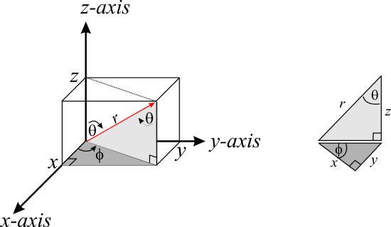
Thus, we use the distance \(r\) of the point from the origin, which is also the magnitude of the vector \(r\), the angle \(\theta\) the vector \(r\) makes with the positive z -axis, and the angle \(\phi\) between the projection of the vector \(r\) into the \(xy\) plane and the positive x -axis. The angle \(\theta\) is called the polar angle and the angle \(\phi\) is called the azimuthal angle . These three variables have the following ranges
\[r \in [0,\infty ) \;\;\;\; \theta \in [0,\pi ] \;\;\;\; \phi \in [0,2\pi ] \label{8.1.2}\]
To map a point from the Cartesian representation \(r=(x,y,z)\) to spherical coordinates \((r, \theta ,\phi )\), a coordinate transformation is needed tells us how points in the two coordinate representations are connected. To determine \(x\) and \(y\), we need the component of \(r\) in the \(xy\) plane, which is \(r\sin\theta \), and its projection into the \(x\) and \(y\) directions, which are
\[\begin{align*}x &= r\sin\theta \cos\phi \\ y &= r\sin \theta \sin \phi \end{align*} \label{8.1.3}\]
Finally, to determine \(z\), we simply need the component of \(r\) along the z-axis, which is \(r\cos\theta \), so
\[z=r\cos\theta \label{8.1.4}\]
These three relations tell us how to map the point \((r,\theta ,\phi )\) into the original Cartesian frame \((x,y,z)\). The inverse of this transformation tells us how to map the Cartesian numbers \((x,y,z)\) back into spherical coordinates. It is simple algebra to show that the inverse is
\[\begin{align*}r &= \sqrt{x^2 +y^2 +z^2}\\ \phi &= \tan^{-1}\dfrac{y}{x}\\ \theta &= \tan^{-1}\dfrac{\sqrt{x^2+y^2}}{z}\end{align*} \label{8.1.5}\]
A note about vectors
Consider a two-dimensional vector \(v\) in the \(xy\) plane. The vector can be represented in terms of its two components \(v=(v_x ,v_y)\). That is, just two numbers \(v_x\) and \(v_y\) are needed, and we know everything about the vector. However, if we know the angle \(\theta\) that \(v\) makes with the x-axis, then we can also use the magnitude \(v=|v|\) and the angle as two alternative numbers that can be used to represent the vector. In this case, since \(v_x =v\cos\theta =|v|\cos\theta \) and \(v_y =v\sin \theta =|v|\sin\theta \), then \(v\) is specified as \(v=(v\cos\theta ,v\sin\theta )\). There is still another alternative scheme for representing \(v\). We can use the magnitude \(v=|v|\) and just one of the components of \(v\). Suppose we wish to represent \(v\) in terms of \(v\) and \(v_x\). since \(v=v_{x}^{2}+v_{y}^{2}\), the other component \(v_y\) is given by \(v_{y}^{2}=v^2 -v_{x}^{2}\), then \(v_y =\sqrt{v^2 -v_{x}^{2}}\), we can write \(v=(v_x ,\sqrt{v^2-v_{x}^{2}})\), which means we only need to know the magnitude \(v\) and one of the components to specify \(v\) entirely. This is the scheme that will be used below to represent the angular momentum, as discussed in the next section.
Angular momentum
In spherical coordinates, the momentum \(p\) of the electron has a radial component \(p_r\), corresponding to motion radially outward from the origin, and an angular component \(L\), corresponding to motion along the surface of a sphere of radius \(r\), i.e. motion perpendicular to the radial direction:
\[p=\left ( p_r, \dfrac{L}{r} \right ) \label{8.1.6}\]
Note that \(L\) is, itself, still a vector, since motion along the surface of a sphere still has more than one component. Its components include motion along the \(\theta\) and along the \(\phi\) directions.
Let us step back briefly into Cartesian components to look at the angular momentum vector \(L\). Its definition is
\[L=r \times p \label{8.1.7}\]
i.e. the vector cross product of \(r\) and \(p\), which is why \(L\) is perpendicular to \(r\). In Cartesian components, \(L\) actually has three components, which are given by
\[\begin{align*}L_x &= yp_z -zp_y \\ L_y &= zp_x -xp_z \\ L_z &= xp_y -yp_x\end{align*} \label{8.1.8}\]
using the definition of the cross product.
The important thing about angular momentum is that if the potential energy \(V\) depends only on \(r\), then angular momentum is conserved. For example, suppose \(V(r)\) is the Coulomb potential, which we will write compactly as
\[V(r)=-\dfrac{k}{r} \label{8.1.9}\]
where \(k=e^2 /(4\pi \epsilon_0 )\). We will show that angular momentum is conserved within the classical mechanical description of the system. If it is true classically, it is also true in quantum mechanics.
The force on the classical electron is
\[F=-\dfrac{k}{r^3}r \label{8.1.10}\]
Therefore, the three force components are
\[F_x =-\dfrac{kx}{r^3}\;\;\;\; F_y =-\dfrac{ky}{r^3}\;\;\;\; F_z =-\dfrac{kz}{r^3} \label{8.1.11}\]
From Newton's second law:
\[F=ma=m\dfrac{dv}{dt}=\dfrac{d(mv)}{dt}=\dfrac{dp}{dt} \label{8.1.12}\]
Now consider one of the components of the angular momentum vector, e.g. \(L_z\). Its time derivative is
\[\begin{align*}\dfrac{dL_z}{dt} &= \dfrac{dx}{dt}p_y +x\dfrac{dp_y}{dt}-\dfrac{dy}{dt}p_x -y\dfrac{dp_x}{dt}\\ &= \dfrac{p_x}{m}p_y +xF_y -\dfrac{p_y}{m}p_x -yF_x \\ &=\dfrac{p_x p_y }{m} -\dfrac{kxy}{r^3} -\dfrac{p_y p_x}{m}+\dfrac{kyx}{r^3} \\ &= 0\end{align*} \label{8.1.13}\]
The same can be shown about \(L_x\) and \(L_y\). Moreover, since \(L^2 =L_{x}^{2}+L_{y}^{2}+L_{z}^{2}\), and the three components \(L_x\), \(L_y\) and \(L_z\) are all constant, \(L^2\) is constant as well.
Thus, both the energy and the angular momentum are conserved in classical mechanics, but classically, both quantities can take on any values. In quantum mechanics, the energy can have only certain allowed values, and because angular momentum is conserved, it too can only have certain allowed values, as Bohr predicted in his model of the hydrogen atom. The allowed energies are
\[E_n = -\dfrac{Z^2 e^4 m_e}{8\epsilon_{0}^{2}h^2}\dfrac{1}{n^2} \label{8.1.14}\]
where \(n=1,2,3,...\)
What about angular momentum? In spherical coordinates, the momentum is \(p=(p_r ,L/r)\), and \(L\) only has two components, one along \(\theta\) and one along \(\phi\). We can assign allowed values to these components separately, however, there is a compelling reason to do things a little differently. In spherical coordinates, the classical energy is given by
\[\dfrac{p_{r}^{2}}{2m_e}+\dfrac{L^2}{2m_e r^2}-\dfrac{Ze^2}{4\pi \epsilon_0 r}=E \label{8.1.15}\]
Thus, \(E\) separates into a purely radial part and an angular part:
\[E=\varepsilon_r +\dfrac{L^2}{2m_e r^2}\]
Note that the energy depends on \(L^2\). since \(L^2\) and each of the three components \(L_x\), \(L_y\) and \(L_z\) are conserved, we can use the representation of \(L\) in which we choose the magnitude \(L\) and one of the components. Why just one component? Note that even though \(L\) has three Cartesian components, it really is only a two dimensional vector since it describes the motion on a two-dimensional surface. Just like the \(xy\) plane is a two-dimensional surface, the surface of a sphere is also two-dimensional, using the angles \(\theta\) and \(\phi\) to locate points on the surface.
The difference is that the surface of a sphere is not flat but curved, so we have to embed it in three-dimensional space. So as a Cartesian representation, three components are needed, but in spherical coordinates, we only need two, i.e. two numbers to represent \(L\). Thus, we can use the magnitude \(L\) and one of its components, which by convention is taken to be the z -component \(L_z\). \(L_z\) describes motion in the \(xy\) plane, i.e. motion in the azimuthal (\(\phi\)) di rection only. However, this is just motion on a ring, so one part of the wave function will just be the particle-on-a-ring wave functions
\[\dfrac{1}{\sqrt{2\pi }}e^{im\phi} \ \label{8.1.17}\]
where \(m=0,\pm 1,\pm 2,...\), and so the allowed values of \(L_z\) are \(m\hbar\).
For \(L^2\), it turns out that the allowed values are
\[L^2 \rightarrow l(l+1)\hbar^2 \label{8.1.18}\]
where \(l\) is an integer that has the range \(l=0,1,2,...,n-1\) in a given energy level characterized by \(n\). Moreover, because \(L_z \leq |L|\), once the value of \(l\) is specified, \(m\) cannot exceed \(l\), so the range of \(m\) is \(m=-l ,-l+1 ,...,l-1,l\).
Schrödinger Equation for the Hydrogen atom and hydrogen-like Cations
The Schrödinger equation for single-electron Coulomb systems in spherical coordinates is
\[-\dfrac{\hbar^2}{2m_e r^2}\left [ r\dfrac{\partial^2}{\partial r^2}(r\psi (r,\theta ,\phi))+\dfrac{1}{\sin\theta }\dfrac{\partial }{\partial \theta}\sin\theta \dfrac{\partial }{\partial \theta}\psi (r,\theta ,\phi )+\dfrac{1}{\sin^2 \theta}\dfrac{\partial^2}{\partial \phi^2}\psi (r, \theta ,\phi) \right ] -\dfrac{Ze^2}{4\pi \epsilon_0 r}\psi (r, \theta ,\phi ) \\=E\psi (r, \theta ,\phi ) \label{Seq}\]
This type of equation is an example of a partial differential equation , which is no simple task to solve. However, solving it gives both the allowed values of the angular momentum discussed above and the allowed energies \(E_n \), which agree with the simpler Bohr model. Thus, we do not need to assume anything except the validity of the Schrödinger equation, and the allowed values of energy and angular momentum, together with the corresponding wavefunctions, all emerge from the solution.
Obviously, we are not going to go through the solution of the Schrödinger equation, but we can understand something about its mechanics and the solutions from a few simple considerations. Remember that the Schrödinger equation is set up starting from the classical energy, which we said takes the form
\[\dfrac{p_{r}^{2}}{2m_e}+\dfrac{L^2}{2m_e r^2}-\dfrac{Ze^2}{4\pi \epsilon_0 r}=E\]
which we can write as
\[E=\varepsilon_r +\dfrac{L^2}{2m_e r^2}\]
where
\[\varepsilon_r =\dfrac{p_{r}^{2}}{2m_e}-\dfrac{Ze^2}{4\pi \epsilon_0 r}\]
The term \(L^2/(2m_e r^2)\) is actually dependent only on \(\theta \) and \(\phi \), so it is purely angular. Given the separability of the energy into radial and angular terms, the wavefunction can be decomposed into a product of the form
\[\psi (r,\theta ,\phi )=R(r)Y(\theta ,\phi )\]
Solution of the angular part for the function \(Y(\theta ,\phi )\) yields the allowed values of the angular momentum \(L^2\) and the z -component \(L_z\). The functions \(Y(\theta ,\phi )\) are then characterized by the integers \(l\) and \(m\), and are denoted \(Y_{lm}(\theta ,\phi )\). They are known as spherical harmonics . Here we present just a few of them for a few values of \(l\).
For \(l=0\), there is just one value of \(m\), \(m=0\), and, therefore, one spherical harmonic, which turns out to be a simple constant:
\[Y_{00}(\theta ,\phi )=\dfrac{1}{\sqrt{4\pi}}\]
For \(l=1\), there are three values of \(m\), \(m=-1,0,1\), and, therefore, three functions \(Y_{1m}(\theta ,\phi )\). These are given by
\[\begin{align*}Y_{11}(\theta ,\phi ) &= -\left ( \dfrac{3}{8\pi} \right )^{1/2}\sin\theta e^{i\phi }\\ Y_{1-1}(\theta ,\phi ) &= \left ( \dfrac{3}{8\pi} \right )^{1/2} \sin\theta e^{-i\phi }\\ Y_{10}(\theta ,\phi ) &= \left ( \dfrac{3}{4\pi } \right )^{1/2}\cos\theta \end{align*}\]
Note: Exponentials of Complex Numbers
Remember that
\[e^{i\phi } = \cos\phi +i\sin\phi\]
\[e^{-i\phi } = \cos\phi -i\sin\phi\]
For \(l=2\), there are five values of \(m\), \(m=-2,-1,0,1,2\), and, therefore, five spherical harmonics, given by
\[\begin{align*}Y_{22}(\theta ,\phi ) &=\left ( \dfrac{15}{32\pi } \right )^{1/2}\sin^2 \theta e^{2i\phi }\\ Y_{2-2}(\theta ,\phi ) &= \left ( \dfrac{15}{32\pi} \right )^{1/2}\sin^2\theta e^{-2i\phi }\\ Y_{21}(\theta ,\phi ) &= -\left ( \dfrac{15}{8\pi } \right )^{1/2}\sin\theta \cos\theta e^{i\phi }\\ Y_{2-1}(\theta ,\phi ) &= \left ( \dfrac{15}{8\pi } \right )^{1/2}\sin\theta \cos\theta e^{-i\phi }\\ Y_{20}(\theta ,\phi ) &= \left ( \dfrac{5}{16\pi} \right )^{1/2} (3\cos^2 \theta -1)\end{align*}\]
The remaining function \(R(r)\) is characterized by the integers \(n\) and \(l\), as this function satisfies the radial part of the Schrödinger equation, also known as the radial Schrödinger equation:
\[-\dfrac{\hbar^2}{2m_e}\dfrac{1}{r}\dfrac{d^2}{dr^2}(rR_{nl}(r))-\dfrac{l(l+1)\hbar^2}{2m_e r^2}R_{nl}(r)-\dfrac{Ze^2}{4\pi \epsilon_0 r}R_{nl}(r)=E_n R_{nl}(r)\]
Note that, while the functions \(Y_{lm}(\theta ,\phi )\) are not particular to the potential \(V(r)\), the radial functions \(R_{nl}(r)\) are particular for the Coulomb potential. It is the solution of the radial Schrödinger equation that leads to the allowed energy levels. The boundary conditions that lead to the quantized energies are \(rR_{nl}(0)=0\) and \(rR_{nl}(\infty )=0\). The radial parts of the wavefunctions that emerge are given by (for the first few values of \(n\) and \(l\) ):
\[\begin{align*}R_{10}(r) &= 2\left ( \dfrac{Z}{a_0} \right )^{3/2}e^{-Zr/a_0}\\ R_{20}(r) &= \dfrac{1}{2\sqrt{2}}\left ( \dfrac{Z}{a_0} \right )^{3/2} \left ( 2-\dfrac{Zr}{a_0} \right ) e^{-Zr/2a_0}\\ R_{21}(r) &= \dfrac{1}{2\sqrt{6}}\left ( \dfrac{Z}{a_0} \right )^{3/2} \dfrac{Zr}{a_0}e^{-Zr/2a_0}\\ R_{30}(r) &= \dfrac{2}{81\sqrt{3}}\left ( \dfrac{Z}{a_0} \right )^{3/2}\left [ 27-18\dfrac{Zr}{a_0}+2 \left ( \dfrac{Zr}{a_0} \right )^2 \right ]e^{-Zr/3a_0}\end{align*}\]
where \(a_0\) is the Bohr radius
\[a_0 = \dfrac{4\pi \epsilon_0 \hbar^2}{e^2 m_e}=0.529177 \times 10^{-10} \ m\]
The full wavefunctions are then composed of products of the radial and angular parts as
\[\psi_{nlm}(r,\theta ,\phi)=R_{nl}(r)Y_{lm}(\theta ,\phi )\]
At this points, several comments are in order. First, the integers \(n,l,m\) that characterize each state are known as the quantum numbers of the system. Each of them corresponds to a quantity that is classically conserved. The number \(n\) is known as the principal quantum number, the number \(l\) is known as the angular quantum number, and the number \(m\) is known as the magnetic quantum number.
As with any quantum system, the wavefunctions \(\psi_{nlm}(r,\theta ,\phi )\) give the probability amplitude for finding the electron in a particular region of space, and these amplitudes are used to compute actual probabilities associated with measurements of the electron's position. The probability of finding the electron in a small volume element \(dV\) of space around the point \(r=(r,\theta ,\phi )\) is
\[\begin{align*}P(electron \ in \ dV \ about \ r,\theta ,\phi ) &= |\psi_{nlm}(r,\theta ,\phi )|^2dV\\ &= R_{nl}^{2}(r)|Y_{lm}(\theta ,\phi)|^2 dV \end{align*}\]
What is \(dV\) ? In Cartesian coordinates, \(dV\) is the volume of a small box of dimensions \(dx\), \(dy\), and \(dz\) in the \(x\), \(y\), and \(z\) directions. That is,
\[dV=dx\,dy\,dz\]
In spherical coordinates, the volume element \(dV\) is a small element of a spherical volume and is given by
\[dV=r^2 \sin \theta\, dr\, d\theta \,d\phi \label{dV}\]
which is derivable from the transformation equations.
Note: 3-D Integration
If we integrate \(dV\) from Equation \(\ref{dV}\) over a sphere of radius \(R\), we should obtain the volume of the sphere:
\[V= \left[\int_0^R r^2 dr\right]\left[\int_0^{\pi}\sin\theta d\theta\right]\left[\int_0^{2\pi}d\phi\right]\]
\[ = \left[\left.{r^3 \over 3}\right\vert _0^R\right]\left[\left.-\cos\theta\right\vert _0^{\pi}\right]\left[\left.\phi\right\vert _0^{2\pi}\right]\]
\[ = {R^3 \over 3}\times 2\times 2\pi\]
\[ = {4 \over 3}\pi R^3\]
which is the formula for the volume of a sphere of radius \(R\).
Example \(\PageIndex{1}\)
The electron in a hydrogen atom \((Z=1)\) is in the state with quantum numbers \(n=1\), \(l=0\) and \(m=0\). What is the probability that a measurement of the electron's position will yield a value \(r\geq 2a_0\)?
Solution
The wavefunction \(\psi_{100}(r,\theta ,\phi )\) is
\[\psi_{100}(r,\theta ,\phi )=\dfrac{2}{a_{0}^{3/2}} \left ( \dfrac{1}{4\pi} \right )^{1/2}e^{-r/a_0}\]
Therefore, the probability we seek is
\[P(r \geq 2a_0 ) = \int_0^{2\pi}\int_0^{\pi}\int_{2a_0}^{\infty} |\psi_{100}(r,\theta ,\phi)|^2 r^2 \sin\,\theta dr\, d\theta \,d\phi\ \]
\[= \dfrac{4}{a_0^{3}}\dfrac{1}{4\pi }\left [ \int_0^{2\pi}d\phi \right ] \left [ \int_0^{\pi} \sin \theta d\theta \right ] \left [ \int_{2a_0}^{\infty}r^2 e^{-2r/a_0}dr \right] \]
\[= \dfrac{1}{a_{0}^3\pi}\cdot 2\pi \cdot 2\int_{2a_0}^{\infty}r^2e^{-2r/a_0}dr \]
Let \(x=2r/a_0\). Then
\[P(r\geq 2a_0)=\dfrac{1}{2}\int_{4}^{\infty}x^2 e^{-x}dx\]
After integrating by parts, we find
\[P(r\geq 2a_0)=13e^{-4}\approx 0.24=24\%\]
which is relatively large given that this is at least two Bohr radii away from the nucleus!
Radial Probability Distribution Functions
The part of the probability involving the product
\[P_{nl}(r)=r^2 R_{nl}^{2}(r) \label{radeq}\]
is known as the radial probability distribution function or simply the radial distribution function . \(P_{nl}(r)dr\) is the probability that a measurement of the electron's position yields a value in a radial shell of thickness \(dr\) and radius \(r\) as shown in the Figure \(\PageIndex{2}\):
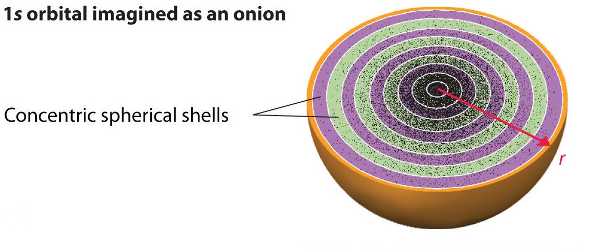
\What the radial probability distribution shows is that the electron cannot be sucked into the nucleus because \(P_{nl}(0)=0\). Hence, as we shrink the radial shell into the nucleus, the probability of finding the electron in that shell goes to 0.
Another point concerns the number of allowed states for each allowed energy. Remember that each wavefunction corresponds to a probability distribution in which the electron can be found for each energy. The more possible states there are, the more varied the electronic properties and behavior of the system will be.
For \(n=1\), there is one energy \(E_1\) and only one wavefunction \(\psi_{100}\).
For \(n=2\), there is one energy \(E_2\) and four possible states, corresponding to the following allowable values of \(l\) and \(m\)
\[\begin{align*} l &= 0 \;\;\;\; m=0\\ l &= 1 \;\;\;\; m=-1,0,1\end{align*}\]
Thus, there are four wavefunctions \(\psi_{200}\), \(\psi_{21-1}\), \(\psi_{210}\), and \(\psi_{211}\).
Note: Degeneracy
Whenever there is more than one wavefunction corresponding to a given energy level, then that energy level is said to be degenerate . In the above example, the \(n=2\) energy level of the hydrogen atom is fourfold degenerate .
Physical Character of the Wavefunctions
The wavefunctions \(\psi_{nlm}(r,\theta ,\phi)\) of the electron are called orbitals, but should not be confused these with trajectories or orbits. These are complete static objects that only give static probabilities when the electron has a well-defined allowable energy. The shapes of the orbitals are largely determined by the values of angular momentum, so we will characterize the orbitals this way.
l=0 orbitals
The \(l=0\) orbitals are called \(s\) (\(s\) for "sharp") orbitals. When \(l=0\), \(m=0\) as well, and the wavefunctions are of the form
\[\psi_{n00}(r,\theta ,\phi )=R_{n0}(r)Y_{00}(\theta ,\phi )=\left ( \dfrac{1}{4\pi} \right )^{1/2}R_{n0}(r)\]
There is no dependence on \(\theta\) or \(\phi\) because \(Y_{00}\) is a constant. Thus, all of these orbitals are spherically symmetric (Figure \(\PageIndex{3}\)).
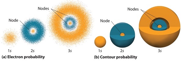
Note several things about these orbitals. First, the density of points dies off exponentially as \(r\) increases, consistent with the exponential dependence of the functions \(R_{n0}(r)\) (Figure \(\PageIndex{4}\)a) .
As \(n\) increases, the exponentials decay more slowly as \(e^{-r/a_0}\) for \(n=1\), \(e^{-r/2a_0}\) for \(n=2\) and \(e^{-r/3a_0}\) for \(n=3\). Note, also, that the wavefunctions are peaked at \(r=0\), which would suggest that the amplitude is maximal to find the electron right on top of the nucleus! In fact, we need to be careful about this interpretation, since the radial probability density (Equation \(\ref{radeq}\)) contains an extra \(r^2\) factor from the volume element which goes to \(0\) as \(r \rightarrow 0\) ( Figure \(\PageIndex{4}\)b ).
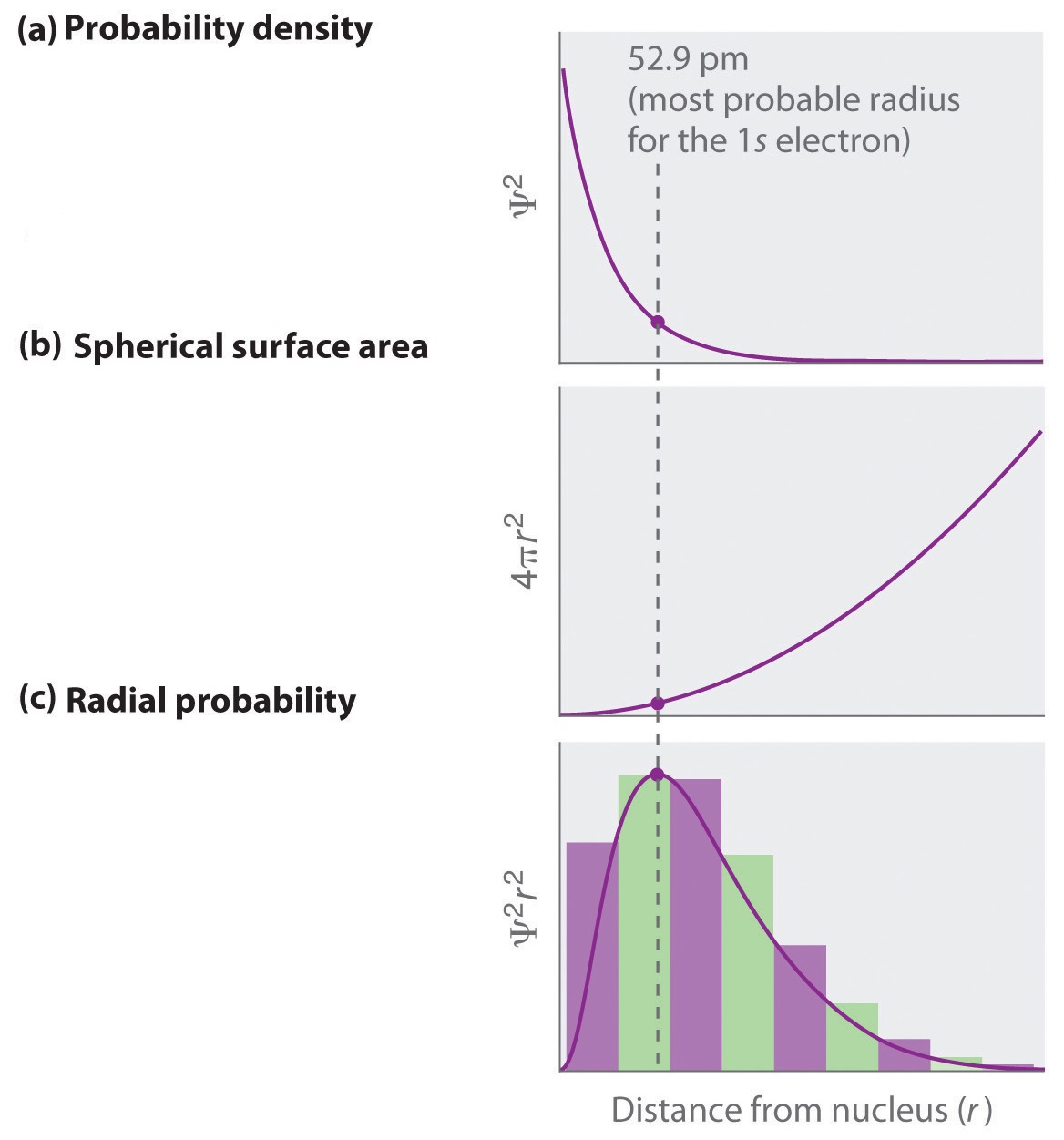
Figure \(\PageIndex{5}\) compares the radial probability densities of the first three \(l=0\) radial wavefunctions.
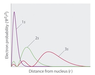
We also see that the wavefunctions have radial nodes where the electron will never be found (Figure \(\PageIndex{5}\)). The number of nodes for \(R_{n0}(r)\) is \(n-1\).
Note: Time Dependence
The Schrödinger Equation (\(\ref{Seq}\)) is often called the time-independent Schrödinger Equation and is limiting case of the more complex time-dependent Schrödinger Equation that includes an explicit dependence to the wavefunction (where the "wave" part is most applicable). This is demonstrated in the simplified "drum" models below for the first three \(l=0\) orbitals.
Simplified 2D drum models of the 1s (left), 2s (middle) and 3s (left) orbitals.
In all of the modes analogous to s orbitals, it can be seen that the center of the \(r=0\) drum vibrates most strongly.
l=1 orbitals
The \(l=1\) orbitals are known as \(p\) (\("p"\) for ``principal'') orbitals. The orbitals take the form
\[\psi_{nlm}(r,\theta ,\phi )=R_{n1}(r)Y_{1m}(\theta ,\phi )\]
where
\[\begin{align*}Y_{1\pm 1}(\theta ,\phi ) &= \pm \left ( \dfrac{3}{8\pi} \right )^{1/2} \sin\theta e^{\pm i\phi }\\ Y_{10}(\theta ,\phi ) &= \left ( \dfrac{3}{4\pi } \right )^{1/2} \cos\theta \end{align*}\]
Thus, these orbitals are not spherically symmetric.
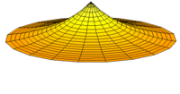
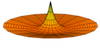
The \(m=0\) orbital is known as the \(p_z\) orbital because of the \(\cos\theta \) dependence and lack of \(\phi \) dependence. This resembles the spherical coordinate transformation for \(z\), \(z=r\cos\theta \). Figure \(\PageIndex{6}\) shows the \(2p\) orbitals in more detail
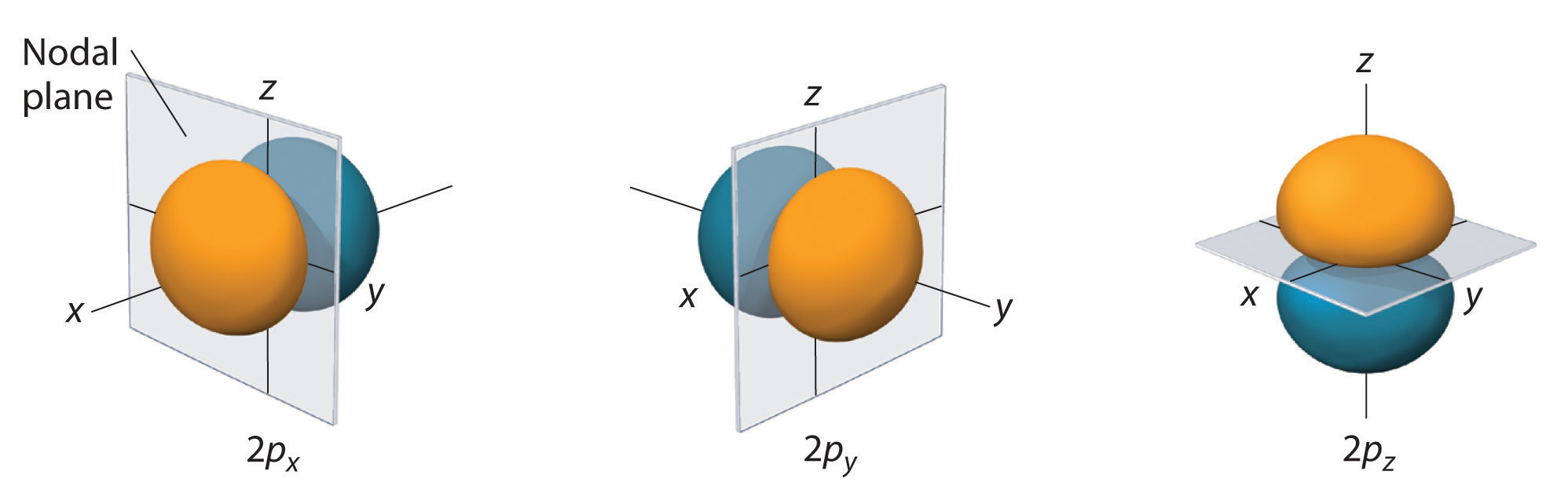
The nodal plane in the \(p\) orbital at \(\theta =\pi /2\) arises because \(\cos(\pi /2)=0\) for all \(\phi\), meaning that the entire \(xy\) plane is a nodal plane.
The orbitals \(\psi_{n11}(r,\theta ,\phi )\) and \(\psi_{n1-1}(r,\theta ,\phi )\) are not real because of the \(exp(\pm i\phi )\) dependence of \(Y_{1\pm 1}(\theta ,\phi )\). Thus, these orbitals are not entire convenient to work with. Fortunately, because \(\psi_{n11}\) and \(\psi_{n1-1}\) are solutions of the Schrödinger equation with the same energy \(E_n\), we can take any combination of these two functions we wish, and we still have a solution of the Schrödinger equation with the same energy. Thus, it is useful to take two combinations that give us two real orbitals. Consider, for example:
\[\begin{align*}\tilde{\psi}_{p_x} &= \dfrac{1}{\sqrt{2}}[\psi_{n1-1}(r,\theta ,\phi )-\psi_{n11}(r,\theta ,\phi )]\\ \tilde{\psi}_{p_y} &= \dfrac{i}{\sqrt{2}}[\psi_{n1-1}(r,\theta ,\phi )+\psi_{n11}(r,\theta ,\phi )]\end{align*}\]
which corresponds to defining new spherical harmonics:
\[\begin{align*}Y_{p_x}(\theta ,\phi ) &= \dfrac{1}{\sqrt{2}}[Y_{1-1}(\theta ,\phi )-Y_{11}(\theta ,\phi )]=\left ( \dfrac{3}{4\pi} \right )^{1/2}\sin\theta \cos\phi \\ Y_{p_y}(\theta ,\phi ) &= \dfrac{i}{\sqrt{2}}[Y_{1-1}(\theta ,\phi )+Y_{11}(\theta ,\phi )]=\left ( \dfrac{3}{4\pi} \right )^{1/2}\sin\theta \sin\phi \end{align*}\]
Again, the notation \(p_x\) and \(p_y\) is used because of the similarity to the spherical coordinate transformations \(x=r\sin\theta \cos\phi \) and \(y=r\sin\theta \sin\phi \). These orbitals have the same shape as the \(p_z\) orbital but are rotated to be oriented along the x -axis for the \(p_x\) orbital and along the y -axis for the \(p_y\) orbital.
l=2 orbitals
The \(l=2\) orbitals are known as \(d\) (\("d"\) for "diffuse") orbitals. Again, we seek combinations of the spherical harmonics that give us real orbitals. The combinations we arrive at are known as \(Y_{xy}\), \(Y_{xz}\), \(Y_{yz}\), \(Y_{z^2}\), \(Y_{x^2 -y^2 }\), which gives us the required five orbitals we need for \(m=-2,-1,0,1,2\). The notation again reflects the angular dependence we would have if we took products \(xy\), \(xz\), \(yz\), \(z^2 \), and \(x^2 -y^2 \) using the spherical coordinate transformation equations.
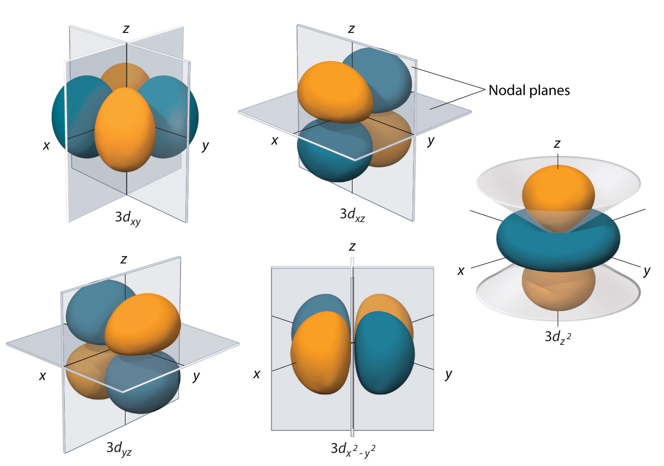
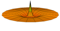
Figure \(\PageIndex{7}\) compared the five \(3d\) orbitals. Note the presence of two nodal planes in most of the orbitals. The exception is the \(3d_{z^2}\) orbital which has a nodal cone. Here, the number of radial nodes is still \(n-l-1\), and, as noted earlier, the overall number of nodes remains the same, so as \(l\) increases, radial nodes are exchanged for angular nodes.
For any of the wavefunctions \(\psi_{nlm}(r,\theta ,\phi )\), the result of measuring the distance of the electron from the nucleus many times yields the average value or expectation value of \(r\), which can be shown to be
\[\begin{align*}\langle r\rangle &= \int_{0}^{2\pi }\int_{0}^{\pi }\int_{0}^{\infty }|\psi_{nlm}(r,\theta ,\phi )|^2 r^3 \sin\theta drd\theta d\phi \\ &= \dfrac{n^2 a_0}{Z}\left [ 1+\dfrac{1}{2}\left ( 1-\dfrac{l(l+1)}{n^2} \right ) \right ]\end{align*}\]