0.5b: Hund's Rules

The Aufbau section discussed how electrons fill the lowest energy orbitals first, and then move up to higher energy orbitals only after the lower energy orbitals are full. However, there is a problem with this rule. Certainly, 1s orbitals should be filled before 2s orbitals, because the 1s orbitals have a lower value of \(n\), and thus a lower energy. What about filling the three different 2p orbitals? In what order should they be filled? The answer to this question involves Hund's rule.

Hund's rule states that:

1. Every orbital in a sublevel is singly occupied before any orbital is doubly occupied.
2. All of the electrons in singly occupied orbitals have the same spin (to maximize total spin).

When assigning electrons to orbitals, an electron first seeks to fill all the orbitals with similar energy (also referred to as degenerate orbitals) before pairing with another electron in a half-filled orbital. Atoms at ground states tend to have as many unpaired electrons as possible. In visualizing this process, consider how electrons exhibit the same behavior as the same poles on a magnet would if they came into contact; as the negatively charged electrons fill orbitals, they first try to get as far as possible from each other before having to pair up.

Example \(\PageIndex{1}\): Nitrogen Atoms

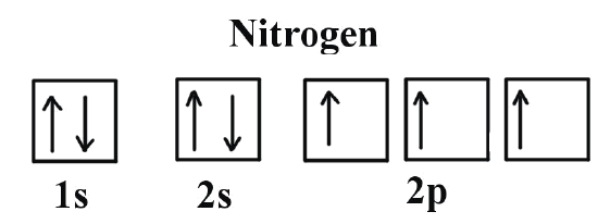
Consider the correct electron configuration of the nitrogen (Z = 7) atom: 1s² 2s² 2p³

The p orbitals are half-filled; there are three electrons and three p orbitals. This is because the three electrons in the 2p subshell will fill all the empty orbitals first before pairing with electrons in them.

Keep in mind that elemental nitrogen is found in nature typically as molecular nitrogen, \(\ce{N2}\), which requires molecular orbitals instead of atomic orbitals as demonstrated above.

Example \(\PageIndex{2}\): Oxygen Atoms

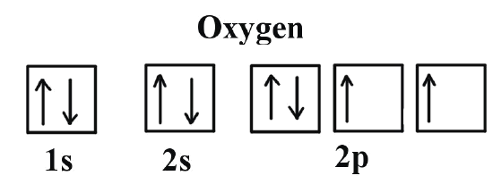
Next, consider oxygen (Z = 8) atom, the element after nitrogen in the same period; its electron configuration is: 1s² 2s² 2p⁴

Oxygen has one more electron than nitrogen; as the orbitals are all half-filled, the new electron must pair up. Keep in mind that elemental oxygen is found in nature typically as molecular oxygen, \(\ce{O_2}\), which has molecular orbitals instead of atomic orbitals as demonstrated above.

Hund's Rule Explained

According to the first rule, electrons always enter an empty orbital before they pair up. Electrons are negatively charged and, as a result, they repel each other. Electrons tend to minimize repulsion by occupying their own orbitals, rather than sharing an orbital with another electron. Furthermore, quantum-mechanical calculations have shown that the electrons in singly occupied orbitals are less effectively screened or shielded from the nucleus. Electron shielding is further discussed in the next section.

For the second rule, unpaired electrons in singly occupied orbitals have the same spins. Technically speaking, the first electron in a sublevel could be either "spin-up" or "spin-down." Once the spin of the first electron in a sublevel is chosen, however, the spins of all of the other electrons in that sublevel depend on that first spin. To avoid confusion, scientists typically draw the first electron, and any other unpaired electron, in an orbital as "spin-up."

Example \(\PageIndex{3}\): Carbon and Oxygen

Consider the electron configuration for carbon atoms: 1s²2s²2p²: The two 2s electrons will occupy the same orbital, whereas the two 2p electrons will be in different orbital (and aligned the same direction) in accordance with Hund's rule.

Consider also the electron configuration of oxygen. Oxygen has 8 electrons. The electron configuration can be written as 1s²2s²2p⁴. To draw the orbital diagram, begin with the following observations: the first two electrons will pair up in the 1s orbital; the next two electrons will pair up in the 2s orbital. That leaves 4 electrons, which must be placed in the 2p orbitals. According to Hund’s rule, all orbitals will be singly occupied before any is doubly occupied. Therefore, two p orbital get one electron and one will have two electrons. Hund's rule also stipulates that all of the unpaired electrons must have the same spin. In keeping with convention, the unpaired electrons are drawn as "spin-up", which gives (Figure 1).

Purpose of Electron Configurations

When atoms come into contact with one another, it is the outermost electrons of these atoms, or valence shell, that will interact first. An atom is least stable (and therefore most reactive) when its valence shell is not full. The valence electrons are largely responsible for an element's chemical behavior. Elements that have the same number of valence electrons often have similar chemical properties.

Electron configurations can also predict stability. An atom is most stable (and therefore unreactive) when all its orbitals are full. The most stable configurations are the ones that have full energy levels. These configurations occur in the noble gases. The noble gases are very stable elements that do not react easily with any other elements. Electron configurations can assist in making predictions about the ways in which certain elements will react, and the chemical compounds or molecules that different elements will form.