9.2: Maxwell’s Equations- Electromagnetic Waves Predicted and Observed

Learning Objectives

• Know the speed of light, and the significance of it related to Maxwell's equations.
• Restate Maxwell’s equations.

At the end of the last chapter we introduced the results of Maxwell's equations. Maxwell made some remarkable and surprising (even to himself!) predictions from these equations. Before looking at these predictions, we must first backtrack to some other information that was known at the time of Maxwell's work: the speed of light.

The Speed of Light

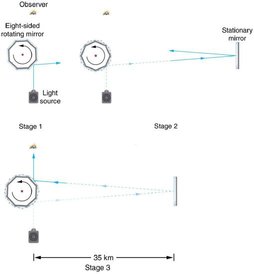
Early attempts to measure the speed of light, such as those made by Galileo, determined that light moved extremely fast, perhaps instantaneously. The first real evidence that light traveled at a finite speed came from the Danish astronomer Ole Roemer in the late 17th century. Roemer had noted that the average orbital period of one of Jupiter’s moons, as measured from Earth, varied depending on whether Earth was moving toward or away from Jupiter. He correctly concluded that the apparent change in period was due to the change in distance between Earth and Jupiter and the time it took light to travel this distance. From his 1676 data, a value of the speed of light was calculated to be \(2.26 \times 10^{8} \mathrm{~m} / \mathrm{s}\) (only 25% different from today’s accepted value). In more recent times, physicists have measured the speed of light in numerous ways and with increasing accuracy. One particularly direct method, used in 1887 by the American physicist Albert Michelson (1852–1931), is illustrated in Figure \(\PageIndex{2}\). Light reflected from a rotating set of mirrors was reflected from a stationary mirror 35 km away and returned to the rotating mirrors. The time for the light to travel can be determined by how fast the mirrors must rotate for the light to be returned to the observer’s eye.

Figure \(\PageIndex{2}\): A schematic of early apparatus used by Michelson and others to determine the speed of light. As the mirrors rotate, the reflected ray is only briefly directed at the stationary mirror. The returning ray will be reflected into the observer's eye only if the next mirror has rotated into the correct position just as the ray returns. By measuring the correct rotation rate, the time for the round trip can be measured and the speed of light calculated. Michelson’s calculated value of the speed of light was only 0.04% different from the value used today.

The speed of light is now known to great precision. In fact, the speed of light in a vacuum \(c\) is so important that it is accepted as one of the basic physical quantities and has the fixed value

\[c=2.9972458 \times 10^{8} \mathrm{~m} / \mathrm{s} \approx 3.00 \times 10^{8} \mathrm{~m} / \mathrm{s}, \nonumber \]

where the approximate value of \(3.00 \times 10^{8} \mathrm{~m} / \mathrm{s}\) is used whenever three-digit accuracy is sufficient.

VALUE OF THE SPEED OF LIGHT

\[c=2.9972458 \times 10^{8} \mathrm{~m} / \mathrm{s} \approx 3.00 \times 10^{8} \mathrm{~m} / \mathrm{s} \nonumber\]

Maxwell's Prediction

Before looking at Maxwell's prediction, let us restate again the results of the equations.

THE RESULTS OF MAXWELL’S EQUATIONS

1. Electric field lines originate on positive charges and terminate on negative charges. The electric field is defined as the force per unit charge on a test charge.
2. Magnetic field lines are continuous, having no beginning or end. No magnetic monopoles are known to exist.
3. A changing magnetic field induces an electric field.
4. Magnetic fields are generated by moving charges or by changing electric fields.

Maxwell’s equations encompass the major laws of electricity and magnetism. What is not so apparent is the symmetry that Maxwell introduced in his mathematical framework. Especially important is his addition of the hypothesis that changing electric fields create magnetic fields. This is exactly analogous (and symmetric) to Faraday’s law of induction and had been suspected for some time, but fits beautifully into Maxwell’s equations.

MAKING CONNECTIONS: UNIFICATION OF FORCES

Maxwell’s complete and symmetric theory showed that electric and magnetic forces are not separate, but different manifestations of the same thing—the electromagnetic force. This classical unification of forces is one motivation for current attempts to unify the four basic forces in nature—the gravitational, electrical, strong, and weak nuclear forces.

Since changing electric fields create relatively weak magnetic fields, they could not be easily detected at the time of Maxwell’s hypothesis. Maxwell realized, however, that oscillating charges, like those in AC circuits, produce changing electric fields. He predicted that these changing fields would propagate from the source like waves generated on a lake by a jumping fish. The waves predicted from this equation would move at a constant velocity, determined only by empirical constants such as the one present in Coulomb's Law. When Maxwell performed this calculation, the results were a very peculiar number: \[3.00 \times 10^{8} \mathrm{~m} / \mathrm{s}. \nonumber \] The most peculiar thing about it was that people already knew this was the speed of light! It wasn't likely a coincidence, these calculations indicated that light itself was a form of this electromagnetic radiation that Maxwell had been hypothesizing.

Other wavelengths should exist—it remained to be seen if they did. If so, Maxwell’s theory and remarkable predictions would be verified, the greatest triumph of physics since Newton. Experimental verification came within a few years, but not before Maxwell’s death.

Hertz’s Observations

The German physicist Heinrich Hertz (1857–1894) was the first to generate and detect certain types of electromagnetic waves in the laboratory. Starting in 1887, he performed a series of experiments that not only confirmed the existence of electromagnetic waves, but also verified that they travel at the speed of light.

Hertz used an AC circuit that resonates at a known frequency and connected it to a loop of wire as shown in Figure \(\PageIndex{2}\). High voltages induced across the gap in the loop produced sparks that were visible evidence of the current in the circuit and that helped generate electromagnetic waves.

Across the laboratory, Hertz had another loop attached to another circuit, which could be tuned (as the dial on a radio) to the same resonant frequency as the first and could, thus, be made to receive electromagnetic waves. This loop also had a gap across which sparks were generated, giving solid evidence that electromagnetic waves had been received.

Figure \(\PageIndex{2}\): The apparatus used by Hertz in 1887 to generate and detect electromagnetic waves. An AC circuit connected to the first loop caused sparks across a gap in the wire loop and generated electromagnetic waves. Sparks across a gap in the second loop located across the laboratory gave evidence that the waves had been received.

Hertz also studied the reflection, refraction, and interference patterns of the electromagnetic waves he generated, verifying their wave character. He was able to determine wavelength from the interference patterns, and knowing their frequency, he could calculate the propagation speed using the equation \(v=f \lambda\) (velocity—or speed—equals frequency times wavelength). Hertz was thus able to prove that electromagnetic waves travel at the speed of light. The SI unit for frequency, the hertz \((1 \mathrm{~Hz}=1 \text { cycle } / \mathrm{sec})\), is named in his honor.

Section Summary

• The speed of light was determined fairly accurately prior to the formulation of Maxwell's equations.
• Electromagnetic waves consist of oscillating electric and magnetic fields and propagate at the speed of light c. They were predicted by Maxwell.
• Maxwell’s prediction of electromagnetic waves resulted from his formulation of a complete and symmetric theory of electricity and magnetism, known as Maxwell’s equations.
• These four equations are paraphrased in this text, rather than presented numerically, and encompass the major laws of electricity and magnetism. First is Gauss’s law for electricity, second is Gauss’s law for magnetism, third is Faraday’s law of induction, including Lenz’s law, and fourth is Ampere’s law in a symmetric formulation that adds another source of magnetism—changing electric fields.
• Hertz verified Maxwell's equations by creating and detecting that radio waves which also moved at the speed of light.

Glossary

electromagnetic waves

radiation in the form of waves of electric and magnetic energy

Maxwell’s equations

a set of four equations that comprise a complete, overarching theory of electromagnetism

hertz

an SI unit denoting the frequency of an electromagnetic wave, in cycles per second

speed of light

in a vacuum, such as space, the speed of light is a constant 3 x 10⁸ m/s

electric field lines

a pattern of imaginary lines that extend between an electric source and charged objects in the surrounding area, with arrows pointed away from positively charged objects and toward negatively charged objects. The more lines in the pattern, the stronger the electric field in that region

magnetic field lines

a pattern of continuous, imaginary lines that emerge from and enter into opposite magnetic poles. The density of the lines indicates the magnitude of the magnetic field