2610 Determination of a Formation Constant

1.0 INTRODUCTION

1.1 Objectives

After completing this experiment, the student will be able to:

• determine the value of the equilibrium constant for formation of FeSCN2+ by using the visible light absorption of the complex ion.
• confirm the stoichiometry of the reaction.

1.2 Background

While some reactions go to completion – and we can calculate the amount of reactants required, products produced, and limiting reagents –, most reactions do not behave this way. Instead, after mixing the reactants, reactions reach a state where a stable mixture of reactants and products is produced. This mixture is called the equilibrium state; at this point, chemical reactions occur in both directions at equal rates. Therefore, once the equilibrium state has been reached, no further change occurs in the concentrations of reactants and products.

We can still determine quantities of chemicals present and the equilibrium constant, Keq, is used to do this. The expression for the equilibrium constant for a reaction is determined by examining the balanced chemical equation. For a reaction involving aqueous reactants and products, the equilibrium constant is expressed as a ratio between reactant and product concentrations, where each term is raised to the power of its reaction coefficient (Equation 1). The ratio chosen gives products over reactants rather than the alternative. When the quantities of reactants and products are given in molar concentrations, the equilibrium constant is referred to as KC. The value of this constant at equilibrium is always the same, regardless of the initial reactant and product concentrations, at a given temperature. Equilibrium constants change with temperature, but at a given temperature, whether the reactants are mixed in their exact stoichiometric ratios, or one reactant is initially present in large excess, the ratio described by the equilibrium constant expression will be achieved once the reaction composition stops changing.

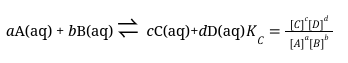(Equation 1)

The reaction to be studied involves the formation of the reddish orange iron(III) thiocyanate complex ion, Fe(H2O)5SCN2+. The actual reaction involves the displacement of a water ligand by thiocyanate ligand, SCN–.

Fe(H2O)63+(aq) + SCN–(aq) ⇌ Fe(H2O)5SCN2+(aq) + H2O(l)

For simplicity, and because water ligands do not change the net charge of the species, water can be omitted from the formulas of Fe(H2O)63+ and Fe(H2O)5SCN2+. Thus, Fe(H2O)63+ is usually written as Fe3+ and Fe(H2O)5SCN2+ is written as FeSCN2+. Also, because the concentration of liquid water is essentially unchanged in aqueous solution, we can write a simpler expression for KC that expresses the equilibrium condition only in terms of species with variable concentrations.

Fe3+(aq) + SCN–(aq) ⇌ FeSCN2+(aq) 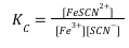(Equation 2)

In this experiment, students will prepare several different aqueous mixtures of Fe3+ and SCN–. Since the reaction reaches equilibrium nearly instantly, these mixtures turn reddish orange very quickly due to the formation of the product, FeSCN2+(aq). The intensity of the color of the mixtures is proportional to the concentration of the product formed at equilibrium. As long as all mixtures are measured at the same temperature, the ratio described in Equation 2 will be the same.

1.2 Measurement of [FeSCN2+] Concentration

Since the complex ion product, FeSCN2+, is the only strongly colored species in the system, its concentration can be determined by measuring the intensity of the orange color in equilibrium systems of the Fe3+, SCN-, and FeSCN2+ ions. You will be using a spectrophotometer and applying Beer’s Law (Equation 3) to do this. The absorbance, A, is directly proportional to two parameters: path length, b (the length of the sample through which the light travels) and C (the molar concentration of the complex ion). Molar absorptivity ε, is a constant that expresses the absorbing ability of a chemical species at a certain wavelength. The absorbance, A, is roughly correlated with the color intensity observed visually; the more intense the color, the higher the absorbance.

A = εbC (Equation 3)

Solutions containing FeSCN2+ are placed into the spectrophotometer and their absorbances at 447 nm are measured. In this method, the path length, b, is the same for all measurements. The value of the combined constants, εb, is determined by plotting the absorbances, A, vs. molar concentrations, C, for several solutions with known concentration of FeSCN2+. The slope of this calibration curve is equal to εb and is then used to find unknown concentrations of FeSCN2+ from their measured absorbances.

1.3 Calculations

In order to determine the value of KC, the equilibrium values of [Fe3+], [SCN–], and [FeSCN2+] must be known. The equilibrium value of [FeSCN2+] is determined spectroscopically. Its initial value will be zero, since no FeSCN2+ will be added to the solution.

The equilibrium values of [Fe3+] and [SCN–] can be determined from a reaction table (ICE table) as shown in Table 1. The initial concentrations of the reactants—that is, [Fe3+] and [SCN–] prior to any reaction—can be found by a dilution calculation based on the values from Table 2 found in the procedure. Once the reaction reaches equilibrium, we assume that the reaction has shifted forward by an amount, x. The equilibrium concentrations of the reactants, Fe3+ and SCN–, are found by subtracting the equilibrium [FeSCN2+] from the initial values. Once all the equilibrium values are known, they can be applied to Equation 2 to determine the value of KC.

Table 1: ICE Table for Determination of Equilibrium Concentrations

	[Fe+3]	[SCN-]	[FeSCN2+]
Initial	[Fe+3]0 (after mixing)	[SCN-]0 (after mixing)	0
Change	- x	- x	+ x
Equilibrium	[Fe+3]0 – x = [Fe+3]0 – [FeSCN2+]S	[SCN-] – x = [SCN-] – [FeSCN2+]S	x = [FeSCN2+]S

[FeSCN2+]S measured spectrophotometrically = Aεb

1.4 Standard Solutions of FeSCN2+

In order to find the equilibrium [FeSCN2+], this experiment requires the preparation of standard solutions with known [FeSCN2+]. These are prepared by mixing a small amount of dilute KSCN solution with a more concentrated solution of Fe(NO3)3. The solution has an overwhelming excess of Fe3+, driving the equilibrium position far towards products. As a result, the equilibrium [Fe3+] is very high due to its large excess, and therefore the equilibrium [SCN–] must be very small. In other words, we can assume that ~100% of the SCN– is reacted, meaning that SCN– is a limiting reactant resulting in the production of an equal amount of FeSCN2+ product. The equilibrium [FeSCN2+] can be approximated as the initial concentration of SCN-, [SCN–]0.

Reference and further reading

Technique I: Use of Spectrophotometer of the laboratory manual

2.0 SAFETY PROCEDURES AND WASTE DISPOSAL

!!Wear your safety goggles!!

The iron(III) nitrate solutions contain nitric acid. Avoid contact with skin and eyes; wash hands frequently during the lab and wash hands and all glassware thoroughly after the experiment.

Collect all your solutions during the lab and dispose of them in the proper waste container.

3.0 CHEMICALS AND SolutionS

Chemical	Concentration	Approximate Amount	Notes
Iron (III) nitrate	2.00 x 10-3 M in 1 M HNO3	30-40 mL
Iron (III) nitrate	0.200 M in 1 M HNO3	25-30 mL
KSCN	2.00 x 10-3 M	15 mL
Laboratory water		25-30 mL

4.0 GLASSWARE AND APPARATUS

Test tubes, large (1) and medium (5)	Spectrophotometer
Stirring rod	Cuvettes (2)
10-mL graduated pipet	5-mL graduated pipet
50-mL or 100-mL beakers (4)

5.0 PROCEDURE

5.1 STOCK Solution, FeSCN2+, PREPARATION FOR STANDARDIZATION

1. Prepare a stock solution with known concentration of FeSCN2+. Obtain 15 mL of 0.200 M Fe(NO3)3 in 1 M HNO3. (Note the actual concentration of this solution.) Rinse your graduated pipet with a few mL of this solution and add 10.00 mL of this solution into a clean and dry small beaker.

2. Using your graduated pipet, add 8.00 mL laboratory water to the small beaker.

3. Rinse your graduated pipet with a few mL of 2.00 x 10–3 M KSCN. Then add 2.00 mL of the KSCN solution to the small beaker.

4. Mix the solution with a clean and dry stirring rod until a uniform dark orange solution is obtained. A few dilutions of the stock solution will be used to prepare four standard solutions for your calibration curve. Calculate the concentrations of these diluted solutions and record on your data recording sheet. In addition, one 'blank' solution containing only Fe(NO3)3 will be used to zero the spectrophotometer (Table 2).

Table 2: Amount of Solutions Needed to Prepare Standards

Standard solutions	Composition of solution
Blank	0.200 M Fe(NO3)3 in 1 M HNO3
1	stock solution
2	4.00 mL stock solution plus 1.00 mL water
3	4.00 mL stock solution plus 2.00 mL water
4	4.00 mL stock solution plus 3.00 mL water

5.2 PREPARATION OF THE EQUILIBRIUM MIXTURES

1. Label two clean and dry 50-mL beaker. Transfer 30-40 mL of 2.00 x 10–3 M Fe(NO3)3 in 1 M HNO3 into one beaker and 25-30 mL of 2.00 x 10–3 M KSCN into the other beaker.

2. Label five clean and dry medium test tubes to be used for the five test mixtures you will make. Using your graduated pipet, add 5.00 mL of 2.00 x 10–3 M Fe(NO3)3 in 1 M HNO3 solution into each of the five test tubes.

3. Using your graduated pipet, add the corresponding amount of KSCN solution to each of the labeled test tubes, according to Table 3 below.

4. Rinse your graduated pipet several times with laboratory water, and then use it to add the appropriate amount of laboratory water into each of the labeled test tubes.

5. Stir each solution thoroughly with your stirring rod until a uniform orange color is obtained. To avoid contaminating the solutions, rinse and dry your stirring rod between each solution preparation.

Table 3: Mixtures of Equilibrium Solutions

Sample	Amount of 2.00 x 10-3 M Fe(NO3)3 in 1 M HNO3	Amount of 2.00 x 10-3 M KSCN	Amount of laboratory water
1	5.00 mL	5.00 mL	0.00 mL
2	5.00 mL	4.00 mL	1.00 mL
3	5.00 mL	3.00 mL	2.00 mL
4	5.00 mL	2.00 mL	3.00 mL
5	5.00 mL	1.00 mL	4.00 mL

5.3 SPECTROPHOTOMETRIC DETERMINATION OF [FeSCN2+]

Review Technique I: Use of Spectrophotometer of the laboratory manual.

1. Fill a cuvette with the blank solution and carefully wipe off the outside with a tissue. Insert the cuvette and make sure it is oriented correctly by aligning the mark on cuvette towards the front. Close the lid. Your instructor will show you how to zero the spectrophotometer with this solution. Set aside this solution for later disposal.

2. For each standard solution in Table 2, rinse your cuvette three times with a small amount (~0.5 mL) of the standard solution to be measured, disposing the rinse solution each time. Then fill the cuvette with the standard, insert the cuvette as before and record the absorbance reading.

3. Finally, repeat this same procedure for the five mixtures with unknown [FeSCN2+] prepared in Part 5.2. The [FeSCN2+] in these solutions will be determined from the calibration curve.

6.0 DATA RECORDING SHEET

Last Name

First Name

Partner Name(s)

Date

1. Absorbances for Standard Solutions from Table 2

Standard solution	[FeSCN+2] (= diluted [SCN-])	Absorbance
1
2
3
4

Show the calculation of [FeSCN+2] (= diluted [SCN-]) for one standard solution below.

2. Initial Reactant Concentrations for Equilibrium Mixture from Table 3

Sample	2.00 x 10-3 M Fe(NO3)3	2.00 x 10-3 M KSCN	Laboratory Water	Initial Concentrations (M)
				Fe3+	SCN–
1	5.00 mL	5.00 mL	0.00 mL
2	5.00 mL	4.00 mL	1.00 mL
3	5.00 mL	3.00 mL	2.00 mL
4	5.00 mL	2.00 mL	3.00 mL
5	5.00 mL	1.00 mL	4.00 mL

Show a dilution calculation for [Fe3+]initial in Sample #1 only.

3. Absorbances for the Equilibrium Mixtures from Table 3.

Sample	Absorbance
1
2
3
4
5

7.0 DATA ANALYSIS

1. Using Microsoft Excel or Google Sheets, plot Absorbance vs. [FeSCN2+] for the standard solutions. Obtain an equation for the line (best-fit). This equation should be in the form, y = mx + b (A = m⋅[FeSCN2+] + constant) and will be used to determine the [FeSCN2+] in the equilibrium mixtures. Attach your graph to this report.

2. Use the equation you obtained from your graph in #1 to determine the [FeSCN2+] in the equilibrium mixtures ([FeSCN2+]equil).

Sample	[FeSCN2+]equil (M)
1
2
3
4
5

Show the calculation of [FeSCN+2]equil for one sample below.

3. Combine the selected information you gathered and complete the table below for all the equilibrium concentrations (see Table 1) and the value of Kc.

Sample	Equilibrium Concentrations (M)			KC
	Fe3+ ([Fe3+]0 - [FeSCN2+])	SCN– ([SCN-]0 - [FeSCN2+])	FeSCN2+
1
2
3
4
5

Average value of KC ________________

(Use reasonable number of significant digits, based on the distribution of your KC values.)

8.0 POST-LAB QUESTIONS

Problem: Is an alternative reaction stoichiometry supported?

Suppose that instead of forming FeSCN2+, the reaction between Fe3+ and SCN– resulted in the formation of Fe(SCN)2+. The reaction analogous to the one in Equation 2 would be:

Fe3+(aq) + 2 SCN–(aq) ⇌ Fe(SCN)2+(aq)

That would mean two moles of SCN– displace two moles of H2O in Fe(H2O)62+, making Fe(SCN)2(H2O)4+.

1. Write the equilibrium constant expression for this reaction.

2. Using the same absorbances for the standard solutions but setting the concentration of the Fe(SCN)2+ equal to ½ of the diluted concentration of SCN- (see Part 6.0 #1), construct a new graph for the calibration curve. Obtain the new equation of the line (best-fit) and provide it below.

(This is because the moles of SCN– assumed to be equal to the moles of complex ion product, FeSCN2+, in our standard solutions. In this alternative reaction, the moles of product, Fe(SCN)2+, equal ½ the number of moles of SCN– added in the standard solutions.)

New equation of the line: ____________________

3. Use this new equation of the line to determine the equilibrium concentration of Fe(SCN)2+ ([Fe(SCN)2+]equil) in each of the sample mixtures and fill in the table below. Remember that since 2 moles of SCN- react in the alternative reaction, [SCN-] at equilibrium is [SCN-]initial – 2[FeSCN2+]equil. The initial concentrations of the Fe3+ and SCN- are the same as before (see Part 6.0 #2).

Sample	Equilibrium Concentrations (M)			KC
	Fe3+ [Fe3+]initial – [Fe(SCN)2+]	SCN– [SCN-]initial – 2[Fe(SCN)2+]	Fe(SCN)2+
1
2
3
4
5

4. Based on the values you got for the KC in this alternative reaction compared to what you calculated assuming only on SCN- reacted, which reaction appears to be correct: one SCN- or two SCN-? Explain your reasoning.