6.2: Similarity Coefficients
- Page ID
- 192635
\( \newcommand{\vecs}[1]{\overset { \scriptstyle \rightharpoonup} {\mathbf{#1}} } \)
\( \newcommand{\vecd}[1]{\overset{-\!-\!\rightharpoonup}{\vphantom{a}\smash {#1}}} \)
\( \newcommand{\dsum}{\displaystyle\sum\limits} \)
\( \newcommand{\dint}{\displaystyle\int\limits} \)
\( \newcommand{\dlim}{\displaystyle\lim\limits} \)
\( \newcommand{\id}{\mathrm{id}}\) \( \newcommand{\Span}{\mathrm{span}}\)
( \newcommand{\kernel}{\mathrm{null}\,}\) \( \newcommand{\range}{\mathrm{range}\,}\)
\( \newcommand{\RealPart}{\mathrm{Re}}\) \( \newcommand{\ImaginaryPart}{\mathrm{Im}}\)
\( \newcommand{\Argument}{\mathrm{Arg}}\) \( \newcommand{\norm}[1]{\| #1 \|}\)
\( \newcommand{\inner}[2]{\langle #1, #2 \rangle}\)
\( \newcommand{\Span}{\mathrm{span}}\)
\( \newcommand{\id}{\mathrm{id}}\)
\( \newcommand{\Span}{\mathrm{span}}\)
\( \newcommand{\kernel}{\mathrm{null}\,}\)
\( \newcommand{\range}{\mathrm{range}\,}\)
\( \newcommand{\RealPart}{\mathrm{Re}}\)
\( \newcommand{\ImaginaryPart}{\mathrm{Im}}\)
\( \newcommand{\Argument}{\mathrm{Arg}}\)
\( \newcommand{\norm}[1]{\| #1 \|}\)
\( \newcommand{\inner}[2]{\langle #1, #2 \rangle}\)
\( \newcommand{\Span}{\mathrm{span}}\) \( \newcommand{\AA}{\unicode[.8,0]{x212B}}\)
\( \newcommand{\vectorA}[1]{\vec{#1}} % arrow\)
\( \newcommand{\vectorAt}[1]{\vec{\text{#1}}} % arrow\)
\( \newcommand{\vectorB}[1]{\overset { \scriptstyle \rightharpoonup} {\mathbf{#1}} } \)
\( \newcommand{\vectorC}[1]{\textbf{#1}} \)
\( \newcommand{\vectorD}[1]{\overrightarrow{#1}} \)
\( \newcommand{\vectorDt}[1]{\overrightarrow{\text{#1}}} \)
\( \newcommand{\vectE}[1]{\overset{-\!-\!\rightharpoonup}{\vphantom{a}\smash{\mathbf {#1}}}} \)
\( \newcommand{\vecs}[1]{\overset { \scriptstyle \rightharpoonup} {\mathbf{#1}} } \)
\(\newcommand{\longvect}{\overrightarrow}\)
\( \newcommand{\vecd}[1]{\overset{-\!-\!\rightharpoonup}{\vphantom{a}\smash {#1}}} \)
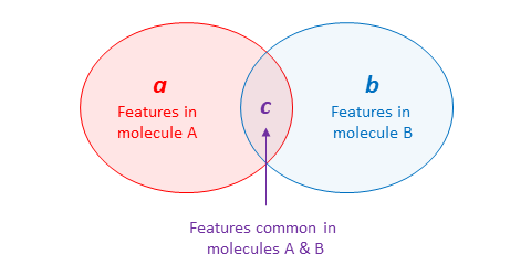
\(\newcommand{\avec}{\mathbf a}\) \(\newcommand{\bvec}{\mathbf b}\) \(\newcommand{\cvec}{\mathbf c}\) \(\newcommand{\dvec}{\mathbf d}\) \(\newcommand{\dtil}{\widetilde{\mathbf d}}\) \(\newcommand{\evec}{\mathbf e}\) \(\newcommand{\fvec}{\mathbf f}\) \(\newcommand{\nvec}{\mathbf n}\) \(\newcommand{\pvec}{\mathbf p}\) \(\newcommand{\qvec}{\mathbf q}\) \(\newcommand{\svec}{\mathbf s}\) \(\newcommand{\tvec}{\mathbf t}\) \(\newcommand{\uvec}{\mathbf u}\) \(\newcommand{\vvec}{\mathbf v}\) \(\newcommand{\wvec}{\mathbf w}\) \(\newcommand{\xvec}{\mathbf x}\) \(\newcommand{\yvec}{\mathbf y}\) \(\newcommand{\zvec}{\mathbf z}\) \(\newcommand{\rvec}{\mathbf r}\) \(\newcommand{\mvec}{\mathbf m}\) \(\newcommand{\zerovec}{\mathbf 0}\) \(\newcommand{\onevec}{\mathbf 1}\) \(\newcommand{\real}{\mathbb R}\) \(\newcommand{\twovec}[2]{\left[\begin{array}{r}#1 \\ #2 \end{array}\right]}\) \(\newcommand{\ctwovec}[2]{\left[\begin{array}{c}#1 \\ #2 \end{array}\right]}\) \(\newcommand{\threevec}[3]{\left[\begin{array}{r}#1 \\ #2 \\ #3 \end{array}\right]}\) \(\newcommand{\cthreevec}[3]{\left[\begin{array}{c}#1 \\ #2 \\ #3 \end{array}\right]}\) \(\newcommand{\fourvec}[4]{\left[\begin{array}{r}#1 \\ #2 \\ #3 \\ #4 \end{array}\right]}\) \(\newcommand{\cfourvec}[4]{\left[\begin{array}{c}#1 \\ #2 \\ #3 \\ #4 \end{array}\right]}\) \(\newcommand{\fivevec}[5]{\left[\begin{array}{r}#1 \\ #2 \\ #3 \\ #4 \\ #5 \\ \end{array}\right]}\) \(\newcommand{\cfivevec}[5]{\left[\begin{array}{c}#1 \\ #2 \\ #3 \\ #4 \\ #5 \\ \end{array}\right]}\) \(\newcommand{\mattwo}[4]{\left[\begin{array}{rr}#1 \amp #2 \\ #3 \amp #4 \\ \end{array}\right]}\) \(\newcommand{\laspan}[1]{\text{Span}\{#1\}}\) \(\newcommand{\bcal}{\cal B}\) \(\newcommand{\ccal}{\cal C}\) \(\newcommand{\scal}{\cal S}\) \(\newcommand{\wcal}{\cal W}\) \(\newcommand{\ecal}{\cal E}\) \(\newcommand{\coords}[2]{\left\{#1\right\}_{#2}}\) \(\newcommand{\gray}[1]{\color{gray}{#1}}\) \(\newcommand{\lgray}[1]{\color{lightgray}{#1}}\) \(\newcommand{\rank}{\operatorname{rank}}\) \(\newcommand{\row}{\text{Row}}\) \(\newcommand{\col}{\text{Col}}\) \(\renewcommand{\row}{\text{Row}}\) \(\newcommand{\nul}{\text{Nul}}\) \(\newcommand{\var}{\text{Var}}\) \(\newcommand{\corr}{\text{corr}}\) \(\newcommand{\len}[1]{\left|#1\right|}\) \(\newcommand{\bbar}{\overline{\bvec}}\) \(\newcommand{\bhat}{\widehat{\bvec}}\) \(\newcommand{\bperp}{\bvec^\perp}\) \(\newcommand{\xhat}{\widehat{\xvec}}\) \(\newcommand{\vhat}{\widehat{\vvec}}\) \(\newcommand{\uhat}{\widehat{\uvec}}\) \(\newcommand{\what}{\widehat{\wvec}}\) \(\newcommand{\Sighat}{\widehat{\Sigma}}\) \(\newcommand{\lt}{<}\) \(\newcommand{\gt}{>}\) \(\newcommand{\amp}{&}\) \(\definecolor{fillinmathshade}{gray}{0.9}\)Many similarity metrics have been proposed and some commonly used metrics in cheminformatics are listed below, along with their mathematical definitions for binary features.

| Metric name | Formula for binary variables |
Minimum | Maximum |
|---|---|---|---|
| Tanimoto (Jaccard) coefficient | 0 | 1 | |
|
Dice coefficient (Hodgkin index) |
0 | 1 | |
| Cosine coefficient (Carbo index) | 0 | 1 | |
| Soergel distance | 0 | 1 | |
| Euclidean distance | 0 | Nα | |
| Hamming (Manhattan or city-block) distance | 0 | Nα |
α The length of molecular fingerprints.
In the above table, the first three metrics (Tanimoto, Dice, and Cosine coefficients) are similarity metrics (SAB), which evaluates how similar two molecules are to each other. The other three (Soergel, Euclidean, and Hamming coefficients) are distance or dissimilarity metrics (DAB), which quantify how dissimilar the molecules are. These dissimilarity measures can be converted into similarity measures in a simple way. For example, for dissimilarity metrics whose possible values range from 0 to 1 (e.g., Soergel distance), the similarity score (SAB) between two molecules can be computed simply by subtracting the dissimilarity score from unity:
Note that the Soergel distance between two molecules is the complement of their Tanimoto coefficient (that is, the sum of the two metrics is 1), while they are developed independently of each other.
If a distance metric has an upper-bound value greater than 1, (e.g., Euclidean or Hamming distance), the following equation [1] can be used to convert the dissimilarity score to the similarity score:
According to this equation, if two molecules are identical to each other, the distance (DAB) between them is zero, and their similarity score (SAB) becomes 1. On the other hand, as the DAB value increases (i.e., for dissimilar molecules), the SAB score approaches to 0.
An important question about molecular similarity evaluation is “how similar is similar?”. To answer this question, it is necessary to have a similarity threshold that can be used to determine whether molecules are similar enough. In 1996, Patterson et al. [2] analyzed sets of active compounds selected from scientific articles and showed that a Tanimoto coefficient of 0.85 or greater reflected a high probability of two compounds having the same activity. Since then, this Tanimoto value of 0.85 has been used in many studies as a general threshold for molecular similarity evaluation. However, as demonstrated in several studies [3], different molecular fingerprints give different similarity score distributions. For example, the Tanimoto score of 0.85 computed from MACCS keys have a different probability of the two compounds sharing the same activity than the probability represented by the same Tanimoto value (0.85) computed from ECFPs. The programming assignments for this chapter will help understand the impact of different molecular fingerprints upon computed similarity coefficient values.
References
- Todeschini R, Ballabio D, Consonni V, Mauri A, Pavan M: CAIMAN (Classification And Influence Matrix Analysis): A new approach to the classification based on leverage-scaled functions. Chemometrics Intell Lab Syst 2007, 87:3-17.
- Patterson DE, Cramer RD, Ferguson AM, Clark RD, Weinberger LE: Neighborhood behavior: A useful concept for validation of ''molecular diversity'' descriptors. J Med Chem 1996, 39:3049-3059.
- Jasial S, Hu Y, Vogt M, Bajorath J: Activity-relevant similarity values for fingerprints and implications for similarity searching [version 2; peer review: 3 approved]. F1000Research 2016, 5

