5.3: Molecular Descriptors
- Page ID
- 192006
\( \newcommand{\vecs}[1]{\overset { \scriptstyle \rightharpoonup} {\mathbf{#1}} } \)
\( \newcommand{\vecd}[1]{\overset{-\!-\!\rightharpoonup}{\vphantom{a}\smash {#1}}} \)
\( \newcommand{\id}{\mathrm{id}}\) \( \newcommand{\Span}{\mathrm{span}}\)
( \newcommand{\kernel}{\mathrm{null}\,}\) \( \newcommand{\range}{\mathrm{range}\,}\)
\( \newcommand{\RealPart}{\mathrm{Re}}\) \( \newcommand{\ImaginaryPart}{\mathrm{Im}}\)
\( \newcommand{\Argument}{\mathrm{Arg}}\) \( \newcommand{\norm}[1]{\| #1 \|}\)
\( \newcommand{\inner}[2]{\langle #1, #2 \rangle}\)
\( \newcommand{\Span}{\mathrm{span}}\)
\( \newcommand{\id}{\mathrm{id}}\)
\( \newcommand{\Span}{\mathrm{span}}\)
\( \newcommand{\kernel}{\mathrm{null}\,}\)
\( \newcommand{\range}{\mathrm{range}\,}\)
\( \newcommand{\RealPart}{\mathrm{Re}}\)
\( \newcommand{\ImaginaryPart}{\mathrm{Im}}\)
\( \newcommand{\Argument}{\mathrm{Arg}}\)
\( \newcommand{\norm}[1]{\| #1 \|}\)
\( \newcommand{\inner}[2]{\langle #1, #2 \rangle}\)
\( \newcommand{\Span}{\mathrm{span}}\) \( \newcommand{\AA}{\unicode[.8,0]{x212B}}\)
\( \newcommand{\vectorA}[1]{\vec{#1}} % arrow\)
\( \newcommand{\vectorAt}[1]{\vec{\text{#1}}} % arrow\)
\( \newcommand{\vectorB}[1]{\overset { \scriptstyle \rightharpoonup} {\mathbf{#1}} } \)
\( \newcommand{\vectorC}[1]{\textbf{#1}} \)
\( \newcommand{\vectorD}[1]{\overrightarrow{#1}} \)
\( \newcommand{\vectorDt}[1]{\overrightarrow{\text{#1}}} \)
\( \newcommand{\vectE}[1]{\overset{-\!-\!\rightharpoonup}{\vphantom{a}\smash{\mathbf {#1}}}} \)
\( \newcommand{\vecs}[1]{\overset { \scriptstyle \rightharpoonup} {\mathbf{#1}} } \)
\( \newcommand{\vecd}[1]{\overset{-\!-\!\rightharpoonup}{\vphantom{a}\smash {#1}}} \)
\(\newcommand{\avec}{\mathbf a}\) \(\newcommand{\bvec}{\mathbf b}\) \(\newcommand{\cvec}{\mathbf c}\) \(\newcommand{\dvec}{\mathbf d}\) \(\newcommand{\dtil}{\widetilde{\mathbf d}}\) \(\newcommand{\evec}{\mathbf e}\) \(\newcommand{\fvec}{\mathbf f}\) \(\newcommand{\nvec}{\mathbf n}\) \(\newcommand{\pvec}{\mathbf p}\) \(\newcommand{\qvec}{\mathbf q}\) \(\newcommand{\svec}{\mathbf s}\) \(\newcommand{\tvec}{\mathbf t}\) \(\newcommand{\uvec}{\mathbf u}\) \(\newcommand{\vvec}{\mathbf v}\) \(\newcommand{\wvec}{\mathbf w}\) \(\newcommand{\xvec}{\mathbf x}\) \(\newcommand{\yvec}{\mathbf y}\) \(\newcommand{\zvec}{\mathbf z}\) \(\newcommand{\rvec}{\mathbf r}\) \(\newcommand{\mvec}{\mathbf m}\) \(\newcommand{\zerovec}{\mathbf 0}\) \(\newcommand{\onevec}{\mathbf 1}\) \(\newcommand{\real}{\mathbb R}\) \(\newcommand{\twovec}[2]{\left[\begin{array}{r}#1 \\ #2 \end{array}\right]}\) \(\newcommand{\ctwovec}[2]{\left[\begin{array}{c}#1 \\ #2 \end{array}\right]}\) \(\newcommand{\threevec}[3]{\left[\begin{array}{r}#1 \\ #2 \\ #3 \end{array}\right]}\) \(\newcommand{\cthreevec}[3]{\left[\begin{array}{c}#1 \\ #2 \\ #3 \end{array}\right]}\) \(\newcommand{\fourvec}[4]{\left[\begin{array}{r}#1 \\ #2 \\ #3 \\ #4 \end{array}\right]}\) \(\newcommand{\cfourvec}[4]{\left[\begin{array}{c}#1 \\ #2 \\ #3 \\ #4 \end{array}\right]}\) \(\newcommand{\fivevec}[5]{\left[\begin{array}{r}#1 \\ #2 \\ #3 \\ #4 \\ #5 \\ \end{array}\right]}\) \(\newcommand{\cfivevec}[5]{\left[\begin{array}{c}#1 \\ #2 \\ #3 \\ #4 \\ #5 \\ \end{array}\right]}\) \(\newcommand{\mattwo}[4]{\left[\begin{array}{rr}#1 \amp #2 \\ #3 \amp #4 \\ \end{array}\right]}\) \(\newcommand{\laspan}[1]{\text{Span}\{#1\}}\) \(\newcommand{\bcal}{\cal B}\) \(\newcommand{\ccal}{\cal C}\) \(\newcommand{\scal}{\cal S}\) \(\newcommand{\wcal}{\cal W}\) \(\newcommand{\ecal}{\cal E}\) \(\newcommand{\coords}[2]{\left\{#1\right\}_{#2}}\) \(\newcommand{\gray}[1]{\color{gray}{#1}}\) \(\newcommand{\lgray}[1]{\color{lightgray}{#1}}\) \(\newcommand{\rank}{\operatorname{rank}}\) \(\newcommand{\row}{\text{Row}}\) \(\newcommand{\col}{\text{Col}}\) \(\renewcommand{\row}{\text{Row}}\) \(\newcommand{\nul}{\text{Nul}}\) \(\newcommand{\var}{\text{Var}}\) \(\newcommand{\corr}{\text{corr}}\) \(\newcommand{\len}[1]{\left|#1\right|}\) \(\newcommand{\bbar}{\overline{\bvec}}\) \(\newcommand{\bhat}{\widehat{\bvec}}\) \(\newcommand{\bperp}{\bvec^\perp}\) \(\newcommand{\xhat}{\widehat{\xvec}}\) \(\newcommand{\vhat}{\widehat{\vvec}}\) \(\newcommand{\uhat}{\widehat{\uvec}}\) \(\newcommand{\what}{\widehat{\wvec}}\) \(\newcommand{\Sighat}{\widehat{\Sigma}}\) \(\newcommand{\lt}{<}\) \(\newcommand{\gt}{>}\) \(\newcommand{\amp}{&}\) \(\definecolor{fillinmathshade}{gray}{0.9}\)If we want to develop a computational model to predict properties, we need to be able to describe them in ways that can be tied to a biological or physical properties. There are many ways that we can represent organic molecules.
Example 1: Representing 2-methylpentane
| 2-methylpentane (IUPAC Name) | Isohexane (synonym) |
CH3CH(CH3)CH2CH2CH3(condensed structure) |
 (Skeletal Line drawing) (Skeletal Line drawing) |
 (Newman projection) (Newman projection) |
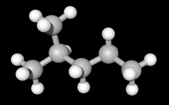
(Ball and Stick Model) |
|
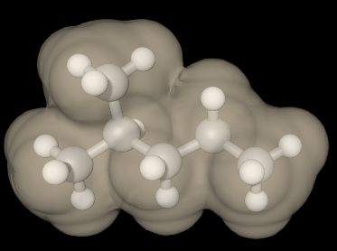
(Van der Waals surface) |
CCCC(C)C (SMILES) |
InChI=1S/C6H14/c1-4-5-6(2)3/h6H,4-5H2,1-3H3 (IUPAC InChI) |
|
AFABGHUZZDYHJO-UHFFFAOYSA-N (IUPAC InChI Key) |
C6H14 (Molecular Formula) |
86.18 g/mol (Molecular weight) |
Each of these representations provides some clue about the nature of the molecule. Some representations can be inferred from others. For example, molecular weight can be calculated from the molecular formula, the SMILES, the condensed structure, or the skeletal drawing. Some representations tell you about the relative position of atoms in either 2D or 3D space. Some of these are inherently easy for humans to read and write, but present challenges for computer processing.
To make a reasonable prediction for any set of molecules, the physical or biological data must be related to the molecule through a series of descriptors. These descriptors can be structural, relating data about the relative position of atoms and types, or calculated data such as electron density using quantum chemical methods.
Descriptors can be classified by the following representations:
|
Molecular representation |
examples |
|
0D |
Atom types, molecular weight, bond types |
|
1D |
Counts of atom types, counts of hydrogen bond donors or acceptors, number of rings, number of functional groups by type |
|
2D |
Mathematical representations by graph theory or calculated values such as lipophilicity or topological polar surface area |
|
3D |
Geometrical descriptors or polar surface area |
In this chapter we will ignore 3D descriptors for now.
0D molecular descriptors
Molecules can be described in a data table by presence or absence or total number of atoms present. The total number of carbon, nitrogen, oxygen or halogen atoms can potentially adequately describe a molecule. For example, in organic chemistry much can be predicted about how a molecule will react or what physical properties it will have just by classifying it as an alkane, an alcohol or an aromatic molecule. Molecular weight in a series of like molecule can be useful to explain difference in boiling points even though that is not fundamental to the property.
1D molecular descriptors
In addition to the types of atoms present, molecules can be further represented by bonding or bonding fragments. Molecules can be described by the number of sp3, sp2, or sp hybridized carbons present. These can also be included in a data table to indicate if they are bonded to an oxygen in the form of an alcohol or a carbonyl. Other functional groups can also be used to adequately describe a molecule by similarity. Indication of presence of C-N, C-S, C=N, or amide or ester functional groups can also tell a lot about how a molecule will interact with solvents or biological systems.
Topological vs topographical descriptors
In cartography, maps are provided that tell you either the relative positions of features on a map (Topological) or the specific distances and elevations of features on a map. For example, public transportation maps usually only represent the stops on a bus or train line, but do not indicate the distance.
Example 2: Topological Map- Metrolink of St. Louis, Missouri https://www.metrostlouis.org/wp-content/uploads/2018/08/MK180468redblueline_update_CORTEX.jpg

A rider can know how many stops are between two points on the map, but not know that the distance between stops may be many miles.
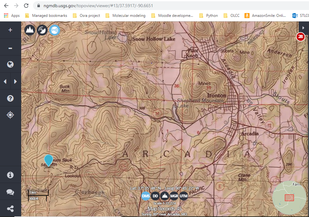
Example 3: Topographical Map- https://ngmdb.usgs.gov/topoview/viewer/#13/37.5917/-90.6651

In this case, a person can know using the scale and the topological lines on the map, how far Taum Sauk Mountain is from Buck Mountain and the elevation change between the two.
Molecules can also be described by topological (two-dimensional 2D) descriptors or topographical (geometrical, three-dimensional 3D) descriptors.
2D Molecular Descriptors
You were introduced to chemical graph theory in section 2.1 of this Libretext. Mathematical notations provide a method for describing chemical structures, and allow for computational processing of molecules in a data set. These are essentially 2D descriptors.
A graph is an abstract structure that contains nodes connected by edges. In representing molecules nodes are the atoms, and edges are the bonds. Hydrogen atoms are usually omitted and thus called “hydrogen depleted molecular graphs.”
Example: Ethane
Note that ethane is described here as a topological map- the connectivity of the molecule is given as relative locations, not exact locations (e.g. atomic size or bond length is excluded).
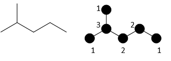
More complicated example- 2-methylpentane
Wiener Index
One of the first mathematical representations of chemical structure used for prediction of properties was developed in 1947 by Harold Weiner. It is defined at the sum of distances between any two carbon atoms (pairs of nodes) in the molecule. Mathematically it is represented as:
Where G represents the total atoms in the molecule, u and v are individual carbon atoms and d(u,v) is the distance in bonds between any two carbon atoms in the shortest path between any two atoms.
In using this index, Weiner showed that the index value is closely correlated with the boiling point of a series of alkanes. Further work also showed that it correlated with other physical properties such as density, surface tension and viscosity.
To calculate the Wiener index for a molecule, for each pair of atoms in the structure, count the distance between atoms. Take the sum of all distances and divide by two. For example in the case of ethane, which only has two nodes:

|
u |
v |
|
|
u |
0 |
1 |
|
v |
1 |
0 |
A more complicated example is pentane:

Pentane has 5 nodes, and distances between each node are calculated and summed.
|
A |
B |
C |
D |
E |
total |
|
|
A |
0 |
1 |
2 |
3 |
4 |
10 |
|
B |
1 |
0 |
1 |
2 |
3 |
7 |
|
C |
2 |
1 |
0 |
1 |
2 |
6 |
|
D |
3 |
2 |
1 |
0 |
1 |
7 |
|
E |
4 |
3 |
2 |
1 |
0 |
10 |
Zagreb Indices
The first and second Zagreb indices (M1 and M2) are another set of classic vertex based descriptors developed in 1972 and 1975, respectively. They were called the Zagreb group indices as their authors were members of the “Rudjer Bošković” Institute in Zagreb, Croatia.
In these indices one counts the connections from each vertex (node, carbon). The first Zagreb index M 1(G) is equal to the sum of squares of the degrees of the vertices, and the second Zagreb index M 2(G) is equal to the sum of the products of the degrees of pairs of adjacent vertices of the underlying molecular graph G.
For pentane, each would be calculated as:

M1 = 12 + 22 + 22 + 22 + 12 = 1 + 4 + 4 + 4 + 1= 14
M2= 1x2 + 2x2 + 2x2 + 2x1 = 2+4+4+2 = 12
For 2-methylpentane, each would be calculated as:

M1 = 12 + 12 + 32 + 22 + 22 + 12 = 1 + 1 + 9+ 4 + 4 + 1= 20
M2 = 1x3 + 1x3 + 3x2 + 2x2 + 2x1 = 3+3+6+4+2 = 18
There are thousands of 2D descriptors that are frequently applied in modeling or predicting properties or biological functions. What is interesting is that these graphs are often descriptors that are reduced to a single value that can be used to make meaning of the physical world.


