3: Quantum Mechanics of Some Simple Systems
- Page ID
- 70774
\( \newcommand{\vecs}[1]{\overset { \scriptstyle \rightharpoonup} {\mathbf{#1}} } \)
\( \newcommand{\vecd}[1]{\overset{-\!-\!\rightharpoonup}{\vphantom{a}\smash {#1}}} \)
\( \newcommand{\dsum}{\displaystyle\sum\limits} \)
\( \newcommand{\dint}{\displaystyle\int\limits} \)
\( \newcommand{\dlim}{\displaystyle\lim\limits} \)
\( \newcommand{\id}{\mathrm{id}}\) \( \newcommand{\Span}{\mathrm{span}}\)
( \newcommand{\kernel}{\mathrm{null}\,}\) \( \newcommand{\range}{\mathrm{range}\,}\)
\( \newcommand{\RealPart}{\mathrm{Re}}\) \( \newcommand{\ImaginaryPart}{\mathrm{Im}}\)
\( \newcommand{\Argument}{\mathrm{Arg}}\) \( \newcommand{\norm}[1]{\| #1 \|}\)
\( \newcommand{\inner}[2]{\langle #1, #2 \rangle}\)
\( \newcommand{\Span}{\mathrm{span}}\)
\( \newcommand{\id}{\mathrm{id}}\)
\( \newcommand{\Span}{\mathrm{span}}\)
\( \newcommand{\kernel}{\mathrm{null}\,}\)
\( \newcommand{\range}{\mathrm{range}\,}\)
\( \newcommand{\RealPart}{\mathrm{Re}}\)
\( \newcommand{\ImaginaryPart}{\mathrm{Im}}\)
\( \newcommand{\Argument}{\mathrm{Arg}}\)
\( \newcommand{\norm}[1]{\| #1 \|}\)
\( \newcommand{\inner}[2]{\langle #1, #2 \rangle}\)
\( \newcommand{\Span}{\mathrm{span}}\) \( \newcommand{\AA}{\unicode[.8,0]{x212B}}\)
\( \newcommand{\vectorA}[1]{\vec{#1}} % arrow\)
\( \newcommand{\vectorAt}[1]{\vec{\text{#1}}} % arrow\)
\( \newcommand{\vectorB}[1]{\overset { \scriptstyle \rightharpoonup} {\mathbf{#1}} } \)
\( \newcommand{\vectorC}[1]{\textbf{#1}} \)
\( \newcommand{\vectorD}[1]{\overrightarrow{#1}} \)
\( \newcommand{\vectorDt}[1]{\overrightarrow{\text{#1}}} \)
\( \newcommand{\vectE}[1]{\overset{-\!-\!\rightharpoonup}{\vphantom{a}\smash{\mathbf {#1}}}} \)
\( \newcommand{\vecs}[1]{\overset { \scriptstyle \rightharpoonup} {\mathbf{#1}} } \)
\(\newcommand{\longvect}{\overrightarrow}\)
\( \newcommand{\vecd}[1]{\overset{-\!-\!\rightharpoonup}{\vphantom{a}\smash {#1}}} \)
\(\newcommand{\avec}{\mathbf a}\) \(\newcommand{\bvec}{\mathbf b}\) \(\newcommand{\cvec}{\mathbf c}\) \(\newcommand{\dvec}{\mathbf d}\) \(\newcommand{\dtil}{\widetilde{\mathbf d}}\) \(\newcommand{\evec}{\mathbf e}\) \(\newcommand{\fvec}{\mathbf f}\) \(\newcommand{\nvec}{\mathbf n}\) \(\newcommand{\pvec}{\mathbf p}\) \(\newcommand{\qvec}{\mathbf q}\) \(\newcommand{\svec}{\mathbf s}\) \(\newcommand{\tvec}{\mathbf t}\) \(\newcommand{\uvec}{\mathbf u}\) \(\newcommand{\vvec}{\mathbf v}\) \(\newcommand{\wvec}{\mathbf w}\) \(\newcommand{\xvec}{\mathbf x}\) \(\newcommand{\yvec}{\mathbf y}\) \(\newcommand{\zvec}{\mathbf z}\) \(\newcommand{\rvec}{\mathbf r}\) \(\newcommand{\mvec}{\mathbf m}\) \(\newcommand{\zerovec}{\mathbf 0}\) \(\newcommand{\onevec}{\mathbf 1}\) \(\newcommand{\real}{\mathbb R}\) \(\newcommand{\twovec}[2]{\left[\begin{array}{r}#1 \\ #2 \end{array}\right]}\) \(\newcommand{\ctwovec}[2]{\left[\begin{array}{c}#1 \\ #2 \end{array}\right]}\) \(\newcommand{\threevec}[3]{\left[\begin{array}{r}#1 \\ #2 \\ #3 \end{array}\right]}\) \(\newcommand{\cthreevec}[3]{\left[\begin{array}{c}#1 \\ #2 \\ #3 \end{array}\right]}\) \(\newcommand{\fourvec}[4]{\left[\begin{array}{r}#1 \\ #2 \\ #3 \\ #4 \end{array}\right]}\) \(\newcommand{\cfourvec}[4]{\left[\begin{array}{c}#1 \\ #2 \\ #3 \\ #4 \end{array}\right]}\) \(\newcommand{\fivevec}[5]{\left[\begin{array}{r}#1 \\ #2 \\ #3 \\ #4 \\ #5 \\ \end{array}\right]}\) \(\newcommand{\cfivevec}[5]{\left[\begin{array}{c}#1 \\ #2 \\ #3 \\ #4 \\ #5 \\ \end{array}\right]}\) \(\newcommand{\mattwo}[4]{\left[\begin{array}{rr}#1 \amp #2 \\ #3 \amp #4 \\ \end{array}\right]}\) \(\newcommand{\laspan}[1]{\text{Span}\{#1\}}\) \(\newcommand{\bcal}{\cal B}\) \(\newcommand{\ccal}{\cal C}\) \(\newcommand{\scal}{\cal S}\) \(\newcommand{\wcal}{\cal W}\) \(\newcommand{\ecal}{\cal E}\) \(\newcommand{\coords}[2]{\left\{#1\right\}_{#2}}\) \(\newcommand{\gray}[1]{\color{gray}{#1}}\) \(\newcommand{\lgray}[1]{\color{lightgray}{#1}}\) \(\newcommand{\rank}{\operatorname{rank}}\) \(\newcommand{\row}{\text{Row}}\) \(\newcommand{\col}{\text{Col}}\) \(\renewcommand{\row}{\text{Row}}\) \(\newcommand{\nul}{\text{Nul}}\) \(\newcommand{\var}{\text{Var}}\) \(\newcommand{\corr}{\text{corr}}\) \(\newcommand{\len}[1]{\left|#1\right|}\) \(\newcommand{\bbar}{\overline{\bvec}}\) \(\newcommand{\bhat}{\widehat{\bvec}}\) \(\newcommand{\bperp}{\bvec^\perp}\) \(\newcommand{\xhat}{\widehat{\xvec}}\) \(\newcommand{\vhat}{\widehat{\vvec}}\) \(\newcommand{\uhat}{\widehat{\uvec}}\) \(\newcommand{\what}{\widehat{\wvec}}\) \(\newcommand{\Sighat}{\widehat{\Sigma}}\) \(\newcommand{\lt}{<}\) \(\newcommand{\gt}{>}\) \(\newcommand{\amp}{&}\) \(\definecolor{fillinmathshade}{gray}{0.9}\)
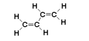
The simple quantum-mechanical problem we have just solved can provide an instructive application to chemistry: the free-electron model (FEM) for delocalized \(\pi\)-electrons. The simplest case is the 1,3-butadiene molecule

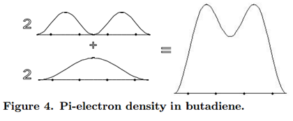
\[\rho =2\psi _{1}^2+2\psi _{2}^2\label{28}\]

A chemical interpretation of this picture might be that, since the \(\pi\)-electron density is concentrated between carbon atoms 1 and 2, and between 3 and 4, the predominant structure of butadiene has double bonds between these two pairs of atoms. Each double bond consists of a \(\pi\)-bond, in addition to the underlying \(\sigma\)-bond. However, this is not the complete story, because we must also take account of the residual \(\pi\)-electron density between carbons 2 and 3. In the terminology of valence-bond theory, butadiene would be described as a resonance hybrid with the contributing structures CH2=CH-CH=CH2 (the predominant structure) and ºCH2-CH=CH-CH2º (a secondary contribution). The reality of the latter structure is suggested by the ability of butadiene to undergo 1,4-addition reactions.
The free-electron model can also be applied to the electronic spectrum of butadiene and other linear polyenes. The lowest unoccupied molecular orbital (LUMO) in butadiene corresponds to the n=3 particle-in-a-box state. Neglecting electron-electron interaction, the longest-wavelength (lowest-energy) electronic transition should occur from n=2, the highest occupied molecular orbital (HOMO).

The energy difference is given by
\[\Delta E=E_{3}-E_{2}=(3^2-2^2)\dfrac{h^2}{8mL^2}\label{29}\]
Here m represents the mass of an electron (not a butadiene molecule!), 9.1x10⁻³¹ Kg, and L is the effective length of the box, 4x1.40x10-10 m. By the Bohr frequency condition
\[\Delta E=h\upsilon =\dfrac{hc}{\lambda }\label{30}\]
The wavelength is predicted to be 207 nm. This compares well with the experimental maximum of the first electronic absorption band, \(\lambda_{max} \approx\) 210 nm, in the ultraviolet region.
We might therefore be emboldened to apply the model to predict absorption spectra in higher polyenes CH2=(CH-CH=)n-1CH2. For the molecule with 2n carbon atoms (n double bonds), the HOMO → LUMO transition corresponds to n → n + 1, thus
\[\dfrac{hc}{\lambda} \approx \begin{bmatrix}(n+1)^2-n^2\end{bmatrix}\dfrac{h^2}{8m(2nL_{CC})^2}\label{31}\]
A useful constant in this computation is the Compton wavelength
\[\dfrac{h}{mc}= 2.426 \times 10^{-12} m.\]
For n=3, hexatriene, the predicted wavelength is 332 nm, while experiment gives \(\lambda _{max}\approx \) 250 nm. For n=4, octatetraene, FEM predicts 460 nm, while \(\lambda _{max}\approx\) 300 nm. Clearly the model has been pushed beyond range of quantitate validity, although the trend of increasing absorption band wavelength with increasing n is correctly predicted. Incidentally, a compound should be colored if its absorption includes any part of the visible range 400-700 nm. Retinol (vitamin A), which contains a polyene chain with n=5, has a pale yellow color. This is its structure:

Contributors and Attributions
Seymour Blinder (Professor Emeritus of Chemistry and Physics at the University of Michigan, Ann Arbor)

