1.7: Errors in Measurement
- Page ID
- 154962
\( \newcommand{\vecs}[1]{\overset { \scriptstyle \rightharpoonup} {\mathbf{#1}} } \)
\( \newcommand{\vecd}[1]{\overset{-\!-\!\rightharpoonup}{\vphantom{a}\smash {#1}}} \)
\( \newcommand{\id}{\mathrm{id}}\) \( \newcommand{\Span}{\mathrm{span}}\)
( \newcommand{\kernel}{\mathrm{null}\,}\) \( \newcommand{\range}{\mathrm{range}\,}\)
\( \newcommand{\RealPart}{\mathrm{Re}}\) \( \newcommand{\ImaginaryPart}{\mathrm{Im}}\)
\( \newcommand{\Argument}{\mathrm{Arg}}\) \( \newcommand{\norm}[1]{\| #1 \|}\)
\( \newcommand{\inner}[2]{\langle #1, #2 \rangle}\)
\( \newcommand{\Span}{\mathrm{span}}\)
\( \newcommand{\id}{\mathrm{id}}\)
\( \newcommand{\Span}{\mathrm{span}}\)
\( \newcommand{\kernel}{\mathrm{null}\,}\)
\( \newcommand{\range}{\mathrm{range}\,}\)
\( \newcommand{\RealPart}{\mathrm{Re}}\)
\( \newcommand{\ImaginaryPart}{\mathrm{Im}}\)
\( \newcommand{\Argument}{\mathrm{Arg}}\)
\( \newcommand{\norm}[1]{\| #1 \|}\)
\( \newcommand{\inner}[2]{\langle #1, #2 \rangle}\)
\( \newcommand{\Span}{\mathrm{span}}\) \( \newcommand{\AA}{\unicode[.8,0]{x212B}}\)
\( \newcommand{\vectorA}[1]{\vec{#1}} % arrow\)
\( \newcommand{\vectorAt}[1]{\vec{\text{#1}}} % arrow\)
\( \newcommand{\vectorB}[1]{\overset { \scriptstyle \rightharpoonup} {\mathbf{#1}} } \)
\( \newcommand{\vectorC}[1]{\textbf{#1}} \)
\( \newcommand{\vectorD}[1]{\overrightarrow{#1}} \)
\( \newcommand{\vectorDt}[1]{\overrightarrow{\text{#1}}} \)
\( \newcommand{\vectE}[1]{\overset{-\!-\!\rightharpoonup}{\vphantom{a}\smash{\mathbf {#1}}}} \)
\( \newcommand{\vecs}[1]{\overset { \scriptstyle \rightharpoonup} {\mathbf{#1}} } \)
\( \newcommand{\vecd}[1]{\overset{-\!-\!\rightharpoonup}{\vphantom{a}\smash {#1}}} \)
\(\newcommand{\avec}{\mathbf a}\) \(\newcommand{\bvec}{\mathbf b}\) \(\newcommand{\cvec}{\mathbf c}\) \(\newcommand{\dvec}{\mathbf d}\) \(\newcommand{\dtil}{\widetilde{\mathbf d}}\) \(\newcommand{\evec}{\mathbf e}\) \(\newcommand{\fvec}{\mathbf f}\) \(\newcommand{\nvec}{\mathbf n}\) \(\newcommand{\pvec}{\mathbf p}\) \(\newcommand{\qvec}{\mathbf q}\) \(\newcommand{\svec}{\mathbf s}\) \(\newcommand{\tvec}{\mathbf t}\) \(\newcommand{\uvec}{\mathbf u}\) \(\newcommand{\vvec}{\mathbf v}\) \(\newcommand{\wvec}{\mathbf w}\) \(\newcommand{\xvec}{\mathbf x}\) \(\newcommand{\yvec}{\mathbf y}\) \(\newcommand{\zvec}{\mathbf z}\) \(\newcommand{\rvec}{\mathbf r}\) \(\newcommand{\mvec}{\mathbf m}\) \(\newcommand{\zerovec}{\mathbf 0}\) \(\newcommand{\onevec}{\mathbf 1}\) \(\newcommand{\real}{\mathbb R}\) \(\newcommand{\twovec}[2]{\left[\begin{array}{r}#1 \\ #2 \end{array}\right]}\) \(\newcommand{\ctwovec}[2]{\left[\begin{array}{c}#1 \\ #2 \end{array}\right]}\) \(\newcommand{\threevec}[3]{\left[\begin{array}{r}#1 \\ #2 \\ #3 \end{array}\right]}\) \(\newcommand{\cthreevec}[3]{\left[\begin{array}{c}#1 \\ #2 \\ #3 \end{array}\right]}\) \(\newcommand{\fourvec}[4]{\left[\begin{array}{r}#1 \\ #2 \\ #3 \\ #4 \end{array}\right]}\) \(\newcommand{\cfourvec}[4]{\left[\begin{array}{c}#1 \\ #2 \\ #3 \\ #4 \end{array}\right]}\) \(\newcommand{\fivevec}[5]{\left[\begin{array}{r}#1 \\ #2 \\ #3 \\ #4 \\ #5 \\ \end{array}\right]}\) \(\newcommand{\cfivevec}[5]{\left[\begin{array}{c}#1 \\ #2 \\ #3 \\ #4 \\ #5 \\ \end{array}\right]}\) \(\newcommand{\mattwo}[4]{\left[\begin{array}{rr}#1 \amp #2 \\ #3 \amp #4 \\ \end{array}\right]}\) \(\newcommand{\laspan}[1]{\text{Span}\{#1\}}\) \(\newcommand{\bcal}{\cal B}\) \(\newcommand{\ccal}{\cal C}\) \(\newcommand{\scal}{\cal S}\) \(\newcommand{\wcal}{\cal W}\) \(\newcommand{\ecal}{\cal E}\) \(\newcommand{\coords}[2]{\left\{#1\right\}_{#2}}\) \(\newcommand{\gray}[1]{\color{gray}{#1}}\) \(\newcommand{\lgray}[1]{\color{lightgray}{#1}}\) \(\newcommand{\rank}{\operatorname{rank}}\) \(\newcommand{\row}{\text{Row}}\) \(\newcommand{\col}{\text{Col}}\) \(\renewcommand{\row}{\text{Row}}\) \(\newcommand{\nul}{\text{Nul}}\) \(\newcommand{\var}{\text{Var}}\) \(\newcommand{\corr}{\text{corr}}\) \(\newcommand{\len}[1]{\left|#1\right|}\) \(\newcommand{\bbar}{\overline{\bvec}}\) \(\newcommand{\bhat}{\widehat{\bvec}}\) \(\newcommand{\bperp}{\bvec^\perp}\) \(\newcommand{\xhat}{\widehat{\xvec}}\) \(\newcommand{\vhat}{\widehat{\vvec}}\) \(\newcommand{\uhat}{\widehat{\uvec}}\) \(\newcommand{\what}{\widehat{\wvec}}\) \(\newcommand{\Sighat}{\widehat{\Sigma}}\) \(\newcommand{\lt}{<}\) \(\newcommand{\gt}{>}\) \(\newcommand{\amp}{&}\) \(\definecolor{fillinmathshade}{gray}{0.9}\)Scientific measurements are of no value (or at least, they're not really scientific) unless they are given with some statement of the errors they contain. If a poll reports that one candidate leads another by 5%, that may be politically useful for the winning candidate to point out. But all respectable polls are scientific, and report errors. If the error in measurement is plus or minus 10%, which indicates anything from the candidate leading by 15% to trailing by 5%, the poll really does not reliably tell who is in the lead. If the poll had an error of 1%, the leading candidate could make a more scientific case that for being in the lead (by a 4% to 6% margin, or 5% +/-1%).
Luckily, we have an easy method for indicating the error in a measurement, and it is suggested in the results we gave for an air-pollution experiment, in which the mass of smoke collected was given as 3.42 × 10⁻² g and the volume of the balloon was given as 1.021 926 4 × 107 cm3.
"Significant Figures"
The volume was calculated from a balloon diameter of 106 inches. There is something strange about the second quantity, though. It contains a number which was copied directly from the display of an electronic calculator and has Too Many Digits to represent the error of measurement properly.
The reliability (more specifically, the random error or precision) of a quantity derived from a measurement is customarily indicated by the number of significant figures (or significant digits) it contains. For example, the three significant digits in the quantity 3.42 × 10⁻² g tell us that a balance was used on which we could distinguish 3.42 × 10⁻² g from 3.43 × 10⁻² or 3.41 × 10⁻² g. There might be some question about the last digit, but those to the left of it are taken as completely reliable. Another way to indicate the same thing is (3.42±0.01) × 10–2 g. Our measurement is somewhere between 3.41 × 10⁻² and 3.43 × 10⁻² g.
To illustrate how the number of significant digits indicates the error, suppose we had a measurement reported as 3.42 g. From the measurement, we would assume an error of 0.01 g, and the percent error is
\[ \text{Percent Error } = \dfrac{\text{Error}}{\text{Value}} \times 100\%\label{1}\]
\[ \text{Percent Error} = \dfrac{0.01 \text{ g}}{3.42 \text{ g}} \times 100\% = 0.29\%\]
If the correctly recorded measurement had more digits, like 3.4275 g, the measurement itself would indicate that a more expensive balance was used to give better precision (a smaller percent error). In this case, the error is 0.0001 g, and the percent error is:
\[ \text{Percent Error} = \dfrac{0.0001 \text{ g}}{3.4265 \text{ g}} \times 100\% = 0.0029\%\]
So we record measurements to the proper number of digits as a rudimentary method[1] for indicating their approximate error.

Figure \(\PageIndex{1}\) The level of a liquid in a graduated cylinder. The saucer-shaped surface of a liquid in a tube is called a meniscus.
Example \(\PageIndex{1}\): Graduated Cylinder
As another example of choosing an appropriate number of significant digits, let us read the volume of liquid in a graduated cylinder.
Solution:
The bottom of the meniscus lies between graduations corresponding to 38 and 39 cm3. We can estimate that it is at 38.5 cm3, but the last digit might be off a bit-perhaps it looks like 38.4 or 38.6 cm3 to you. Since the third digit is in question, we should use three significant figures. The volume would be recorded as 38.5 cm3, indicating 0.1 cm3 error. Laboratory equipment is often calibrated similarly to this graduated cylinder—you should estimate to the nearest tenth of the smallest graduation.
Counting Significant Digits
In some ordinary numbers, for example, 0.001 23, zeros serve merely to locate the decimal point. They do not indicate the reliability of the measurement and therefore are not significant. Another advantage of scientific notation is that we can assume that all digits are significant. Thus if 0.001 23 is written as 1.23 × 10⁻³, only the 1, 2, and 3, which indicate the reliability of the measurement, are written. The decimal point is located by the power of 10.
If the rule expressed in the previous paragraph is applied to the volume of air collected in our pollution experiment, 1.021 926 4 × 107 cm3, we find that the volume has eight significant digits. This implies that it was determined to ±1 cm3 out of about 10 million cm3, a reliability which corresponds to locating a grasshopper exactly at some point along the road from Philadelphia to New York City. For experiments as crude as ours, this is not likely. Let us see just how good the measurement was.
You will recall that we calculated the volume from the diameter of the balloon, 106 in. The three significant figures imply that this might have been as large as 107 in or as small as 105 in. We can repeat the calculation with each of these quantities to see how far off the volume would be:
\(\begin{align} & \text{ }r\text{ = }\dfrac{\text{1}}{\text{2}}\text{ }\times \text{ 107 in = 53}\text{.5 in }\times \text{ }\dfrac{\text{1 cm}}{\text{0}\text{.3937 in}}\text{ } \\ & \text{ = 135}\text{.890 27 cm} \\ & \text{ }V\text{ = }\dfrac{\text{4}}{\text{3}}\text{ }\times \text{ 3}\text{.141 59 }\times \text{ (135}\text{.890 27 cm)}^{\text{3}}\text{ } \\ & \text{ = 10 511 225 cm}^{\text{3}}\text{ = 1}\text{.051 122 5 }\times \text{ 10}^{\text{7}}\text{ cm}^{\text{3}} \\ & \text{or }V\text{ = }\dfrac{\text{4}}{\text{3}}\text{ }\times \text{ 3}\text{.141 59 }\times \text{ }\left( \dfrac{\text{1}}{\text{2}}\text{ }\times \text{ 105 in }\times \text{ }\dfrac{\text{1 cm}}{\text{0}\text{.3937 in}} \right)^{\text{3}}\text{ } \\ & \text{ = 9 932 759 cm}^{\text{3}}\text{ = 0}\text{.993 275 9 }\times \text{ 10}^{\text{7}}\text{ cm}^{\text{3}} \\ \end{align}\)
That is, the volume is between 0.99 × 10⁷ and 1.05 × 107 cm3 or (1.02 ± 0.03) × 107 cm3. We should round our result to three significant figures, for example, 1.02 cm³, because the last digit, namely 2, is in question.
So the conclusion is simple: The calculated result cannot be more precise than the measurement from which it was made. To show this in an alternative way, the error in 106 in would be about 1 in, so the percent error is
\[ \text{Percent Error} = \dfrac{1 \text{ in}}{106 \text{ in}} \times 100\% = 0.9\%\]
If the result is reported as 10 219 264 cm3, the implied error is 1 part in 10 219 264 and the percent error is:
\[ \text{Percent Error} = \dfrac{1 \text{ cm}^{\text{3}}}{10219264 \text{ cm}^\text{3}} \times 100\% = 0.000009\%\]
Clearly, we should not be able to increase the precision of our data by merely manipulating the data mathematically, so we need simple rules for rounding numbers in calculated quantities.
If the result is reported properly as 1.02 × 107 cm3, the percent error is
-
- \[ \text{Percent Error} = \dfrac{0.01 \text{ cm}^{\text{3}}}{1.02 \text{ cm}^\text{3}} \times 100\% = 1\%\],
approximately the same as the original measurement.
Rules for Rounding Numbers
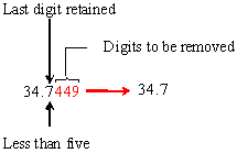
- All digits to be rounded are removed together, not one at a time.
- If the left-most digit to be removed is less than five, the last digit retained is not altered.
- If the left-most digit to be removed is greater than five, the last digit retained is increased by one.
- If the left-most digit to be removed is five and at least one of the other digits to be removed is nonzero. the last digit retained is increased by one.
- If the left-most digit to he removed is five and all other digits to he removed are zero, the last digit retained is not altered if it is even, but is increased by one if it is odd.
Application of the Rules for Rounding Numbers can be illustrated by an example.
Example \(\PageIndex{2}\) : Rounding
Round each of the numbers below to three significant figures.
a) 34.7449 b) 34.864 c) 34.754 d) 34.250 e) 34.35
Solution
a) Apply rules 1 and 2:

(Note that a different result would be obtained if the digits were incorrectly rounded one at a time from the right.)
b) Apply rules 1 and 3: 34.864 → 34.9
c) Apply rules 1 and 4: 34.754 → 34.8
d) Apply rules 1 and 5: 34.250 → 34.2
e) Apply rule 5: 34.35 → 34.4
Example \(\PageIndex{2}\) : Rounding
Round each of the numbers below to three significant figures.
a) 34.7449 b) 34.864 c) 34.754 d) 34.250 e) 34.35
Solution
a) Apply rules 1 and 2:

(Note that a different result would be obtained if the digits were incorrectly rounded one at a time from the right.)
b) Apply rules 1 and 3: 34.864 → 34.9c) Apply rules 1 and 4: 34.754 → 34.8
d) Apply rules 1 and 5: 34.250 → 34.2
e) Apply rule 5: 34.35 → 34.4
To how many significant figures should we round our air-pollution results? We have already done a calculation involving multiplication and division to obtain the volume of our gas-collection balloon. It involved the following quantities and numbers:
| \( 106 \text{ in}\) | A measured quantity with three significant figures |
| \( 0.3937 \text{ in/cm}\) | A conversion factor given with four significant figures(1) |
| \(3.141 59\) | π used with six significant figures (we could obtain more if we wanted) |
| \(\tfrac{\text{4}}{\text{3}} \text{ and } \tfrac{\text{1}}{\text{2}}\) | Numbers(2) with an infinite number of significant figures since the integers in these fractions are exact by definition |
- some conversion factors like 1 mg = 0.001 g are exact, and have an infinite number of significant figures).
- Note that pure numbers are not measurements or quantities, and so they are unlimited in the number of significant figures (numbers have zero error).
The result of the calculation contained three significant figures — the same as the least-reliable number. This illustrates the general rule that for multiplication and division the number of significant figures in the result is the same as in the least-reliable measurement. Defined numbers such as π, ½ or 100 cm/1m are assumed to have an infinite number of significant figures.
In the case of addition and subtraction, a different rule applies. Suppose, for example, that we weighed a smoke-collection filter on a relatively inaccurate balance that could only be read to the nearest 0.01 g. After collecting a sample, the filter was reweighed on a single-pan balance to determine the mass of smoke particles.
- Final mass: 2.3745 g (colored digits are in question)
- Initial mass: –2.32 g
- Mass of smoke: 0.0545 g
Since the initial weighing could have been anywhere from 2.31 to 2.33 g, all three figures in the final result are in question. (It must be between 0.0445 and 0.0645 g). Thus there is but one significant digit, and the result is 0.05g. The rule here is that the result of addition or subtraction cannot contain more digits to the right than there are in any of the numbers added or subtracted. Note that subtraction can drastically reduce the number of significant digits when this rule is applied.
Rounding numbers is especially important if you use an electronic calculator, since these machines usually display a large number of digits, most of which are meaningless. The best procedure is to carry all digits to the end of the calculation (your calculator will not mind the extra work!) and then round appropriately. Answers to subsequent calculations in this book will be rounded according to the rules given. You may wish to go back to previous examples and round their answers correctly as well.
Example \(\PageIndex{3}\): Significant Figures
Evaluate the following expressions, rounding the answer to the appropriate number of significant figures.
- \(32.61 \text{g} + 8.446 \text{g} + 7.0 \text{g} \)
- \(0.136 \text{cm}^3 \times 10.685 \text{g cm}^{-3}\)
Solution
- \(32.61 \text{g} + 8.446 \text{g} + 7.0 \text{g} = 48.056 \text{g} = 48.1 \text{g (7.0 has only one figure to the right of the decimal point.)}\)
- \(0.136 \text{cm}^3 \times 10.685 \text{g cm}^{-3} = 1.453 \text{g} = 1.45 \text{g (0.136 has only three significant figures.)}\)
Precision vs. Accuracy
When we suggested filling a surplus weather balloon to measure how much gas was pumped through our air-pollution collector, we mentioned that this would be a rather crude way to determine volume. For one thing, it would not be all that simple to measure the diameter of an 8- or 9-ft sphere reliably. Using a yardstick, we would be lucky to have successive measurements agree within half an inch or so. It was for this reason that the result was reported to the nearest inch. The degree to which repeated measurements of the same quantity yield the same result is called precision. Repetition of a highly precise measurement would yield almost identical results, whereas low precision implies numbers would differ by a significant percentage from each other.
A highly precise measurement of the diameter of our balloon could be achieved, but it would probably not be worthwhile. We have assumed a spherical shape, but this is almost certainly not exactly correct. No matter how precisely we determine the diameter, our measurement of gas volume will be influenced by deviations from the assumed shape. When one or more of our assumptions about a measuring instrument are wrong, the accuracy of a result will be affected. An obvious example would be a foot rule divided into 11 equal inches. Measurements employing this instrument might agree very precisely, but they would not be very accurate. The following data on the mass of the smoke, measured repeatedly with two balances and a scale, show the difference between accuracy and precision. If he mass has been determined to be exactly 0.03420 g by an independent measurement, the first balance is both accurate (the correct value is obtained) and precise (the range of measurements is small); the second balance is precise, but not accurate; the scale is neither accurate nor precise. Note that we are comparing the three to one another; relative to a balance that had a range of 0.00001 g, all three would be imprecise.
| Mass, Balance A | Mass, Balance B | Mass, Scale | |
|---|---|---|---|
| 0.0342 | 0.0362 | 0.0380 | |
| 0.0341 | 0.0361 | 0.0370 | |
| 0.0342 | 0.0363 | 0.0390 | |
| 0.0343 | 0.0362 | 0.0400 | |
| average | 0.0342 | 0.0362 | 0.0385 |
| range | 0.001 | 0.001 | 0.013 |
The following figures help to understand the difference between precision (small expected difference between multiple measurements) and accuracy (difference between the result and a known value).


Figure \(\PageIndex{1}\): a) High accuracy, Low Precision b)High precision, Low accuracy
An important point of a different kind is illustrated in the last two paragraphs. A great many common words have been adopted into the language of science. Usually such an adoption is accompanied by an unambiguous scientific definition which does not appear in a normal dictionary. Precision and accuracy are many times treated as synonyms, but in science each has a slightly different meaning. Another example is quantity, which we have defined in terms of “number × unit.” Other English words like bulk, size, amount, and so forth, may be synonymous with quantity in everyday speech, but not in science. As you encounter other words like this, try to learn and use the scientific definition as soon as possible, and avoid confusing it with the other meanings you already know.
Even granting the crudeness of the measurements we have just described, they would be adequate to demonstrate whether or not an air-pollution problem existed. The next step would be to find a chemist or public health official who was an expert in assessing air quality, present your data, and convince that person to lend his or her skill and authority to your contention that something was wrong. Such a person would have available equipment whose precision and accuracy were adequate for highly reliable measurements and would be able to make authoritative public statements about the extent of the air-pollution problem.
Contributors
Ed Vitz (Kutztown University), John W. Moore (UW-Madison), Justin Shorb (Hope College), Xavier Prat-Resina (University of Minnesota Rochester), Tim Wendorff, and Adam Hahn.


