10.3: The Gas Laws
- Page ID
- 55012
\( \newcommand{\vecs}[1]{\overset { \scriptstyle \rightharpoonup} {\mathbf{#1}} } \)
\( \newcommand{\vecd}[1]{\overset{-\!-\!\rightharpoonup}{\vphantom{a}\smash {#1}}} \)
\( \newcommand{\dsum}{\displaystyle\sum\limits} \)
\( \newcommand{\dint}{\displaystyle\int\limits} \)
\( \newcommand{\dlim}{\displaystyle\lim\limits} \)
\( \newcommand{\id}{\mathrm{id}}\) \( \newcommand{\Span}{\mathrm{span}}\)
( \newcommand{\kernel}{\mathrm{null}\,}\) \( \newcommand{\range}{\mathrm{range}\,}\)
\( \newcommand{\RealPart}{\mathrm{Re}}\) \( \newcommand{\ImaginaryPart}{\mathrm{Im}}\)
\( \newcommand{\Argument}{\mathrm{Arg}}\) \( \newcommand{\norm}[1]{\| #1 \|}\)
\( \newcommand{\inner}[2]{\langle #1, #2 \rangle}\)
\( \newcommand{\Span}{\mathrm{span}}\)
\( \newcommand{\id}{\mathrm{id}}\)
\( \newcommand{\Span}{\mathrm{span}}\)
\( \newcommand{\kernel}{\mathrm{null}\,}\)
\( \newcommand{\range}{\mathrm{range}\,}\)
\( \newcommand{\RealPart}{\mathrm{Re}}\)
\( \newcommand{\ImaginaryPart}{\mathrm{Im}}\)
\( \newcommand{\Argument}{\mathrm{Arg}}\)
\( \newcommand{\norm}[1]{\| #1 \|}\)
\( \newcommand{\inner}[2]{\langle #1, #2 \rangle}\)
\( \newcommand{\Span}{\mathrm{span}}\) \( \newcommand{\AA}{\unicode[.8,0]{x212B}}\)
\( \newcommand{\vectorA}[1]{\vec{#1}} % arrow\)
\( \newcommand{\vectorAt}[1]{\vec{\text{#1}}} % arrow\)
\( \newcommand{\vectorB}[1]{\overset { \scriptstyle \rightharpoonup} {\mathbf{#1}} } \)
\( \newcommand{\vectorC}[1]{\textbf{#1}} \)
\( \newcommand{\vectorD}[1]{\overrightarrow{#1}} \)
\( \newcommand{\vectorDt}[1]{\overrightarrow{\text{#1}}} \)
\( \newcommand{\vectE}[1]{\overset{-\!-\!\rightharpoonup}{\vphantom{a}\smash{\mathbf {#1}}}} \)
\( \newcommand{\vecs}[1]{\overset { \scriptstyle \rightharpoonup} {\mathbf{#1}} } \)
\(\newcommand{\longvect}{\overrightarrow}\)
\( \newcommand{\vecd}[1]{\overset{-\!-\!\rightharpoonup}{\vphantom{a}\smash {#1}}} \)
\(\newcommand{\avec}{\mathbf a}\) \(\newcommand{\bvec}{\mathbf b}\) \(\newcommand{\cvec}{\mathbf c}\) \(\newcommand{\dvec}{\mathbf d}\) \(\newcommand{\dtil}{\widetilde{\mathbf d}}\) \(\newcommand{\evec}{\mathbf e}\) \(\newcommand{\fvec}{\mathbf f}\) \(\newcommand{\nvec}{\mathbf n}\) \(\newcommand{\pvec}{\mathbf p}\) \(\newcommand{\qvec}{\mathbf q}\) \(\newcommand{\svec}{\mathbf s}\) \(\newcommand{\tvec}{\mathbf t}\) \(\newcommand{\uvec}{\mathbf u}\) \(\newcommand{\vvec}{\mathbf v}\) \(\newcommand{\wvec}{\mathbf w}\) \(\newcommand{\xvec}{\mathbf x}\) \(\newcommand{\yvec}{\mathbf y}\) \(\newcommand{\zvec}{\mathbf z}\) \(\newcommand{\rvec}{\mathbf r}\) \(\newcommand{\mvec}{\mathbf m}\) \(\newcommand{\zerovec}{\mathbf 0}\) \(\newcommand{\onevec}{\mathbf 1}\) \(\newcommand{\real}{\mathbb R}\) \(\newcommand{\twovec}[2]{\left[\begin{array}{r}#1 \\ #2 \end{array}\right]}\) \(\newcommand{\ctwovec}[2]{\left[\begin{array}{c}#1 \\ #2 \end{array}\right]}\) \(\newcommand{\threevec}[3]{\left[\begin{array}{r}#1 \\ #2 \\ #3 \end{array}\right]}\) \(\newcommand{\cthreevec}[3]{\left[\begin{array}{c}#1 \\ #2 \\ #3 \end{array}\right]}\) \(\newcommand{\fourvec}[4]{\left[\begin{array}{r}#1 \\ #2 \\ #3 \\ #4 \end{array}\right]}\) \(\newcommand{\cfourvec}[4]{\left[\begin{array}{c}#1 \\ #2 \\ #3 \\ #4 \end{array}\right]}\) \(\newcommand{\fivevec}[5]{\left[\begin{array}{r}#1 \\ #2 \\ #3 \\ #4 \\ #5 \\ \end{array}\right]}\) \(\newcommand{\cfivevec}[5]{\left[\begin{array}{c}#1 \\ #2 \\ #3 \\ #4 \\ #5 \\ \end{array}\right]}\) \(\newcommand{\mattwo}[4]{\left[\begin{array}{rr}#1 \amp #2 \\ #3 \amp #4 \\ \end{array}\right]}\) \(\newcommand{\laspan}[1]{\text{Span}\{#1\}}\) \(\newcommand{\bcal}{\cal B}\) \(\newcommand{\ccal}{\cal C}\) \(\newcommand{\scal}{\cal S}\) \(\newcommand{\wcal}{\cal W}\) \(\newcommand{\ecal}{\cal E}\) \(\newcommand{\coords}[2]{\left\{#1\right\}_{#2}}\) \(\newcommand{\gray}[1]{\color{gray}{#1}}\) \(\newcommand{\lgray}[1]{\color{lightgray}{#1}}\) \(\newcommand{\rank}{\operatorname{rank}}\) \(\newcommand{\row}{\text{Row}}\) \(\newcommand{\col}{\text{Col}}\) \(\renewcommand{\row}{\text{Row}}\) \(\newcommand{\nul}{\text{Nul}}\) \(\newcommand{\var}{\text{Var}}\) \(\newcommand{\corr}{\text{corr}}\) \(\newcommand{\len}[1]{\left|#1\right|}\) \(\newcommand{\bbar}{\overline{\bvec}}\) \(\newcommand{\bhat}{\widehat{\bvec}}\) \(\newcommand{\bperp}{\bvec^\perp}\) \(\newcommand{\xhat}{\widehat{\xvec}}\) \(\newcommand{\vhat}{\widehat{\vvec}}\) \(\newcommand{\uhat}{\widehat{\uvec}}\) \(\newcommand{\what}{\widehat{\wvec}}\) \(\newcommand{\Sighat}{\widehat{\Sigma}}\) \(\newcommand{\lt}{<}\) \(\newcommand{\gt}{>}\) \(\newcommand{\amp}{&}\) \(\definecolor{fillinmathshade}{gray}{0.9}\)- To understand the relationships among pressure, temperature, volume, and the amount of a gas.
Early scientists explored the relationships among the pressure of a gas (P) and its temperature (T), volume (V), and amount (n) by holding two of the four variables constant (amount and temperature, for example), varying a third (such as pressure), and measuring the effect of the change on the fourth (in this case, volume). The history of their discoveries provides several excellent examples of the scientific method.
The Relationship between Pressure and Volume: Boyle's Law
As the pressure on a gas increases, the volume of the gas decreases because the gas particles are forced closer together. Conversely, as the pressure on a gas decreases, the gas volume increases because the gas particles can now move farther apart. Weather balloons get larger as they rise through the atmosphere to regions of lower pressure because the volume of the gas has increased; that is, the atmospheric gas exerts less pressure on the surface of the balloon, so the interior gas expands until the internal and external pressures are equal.

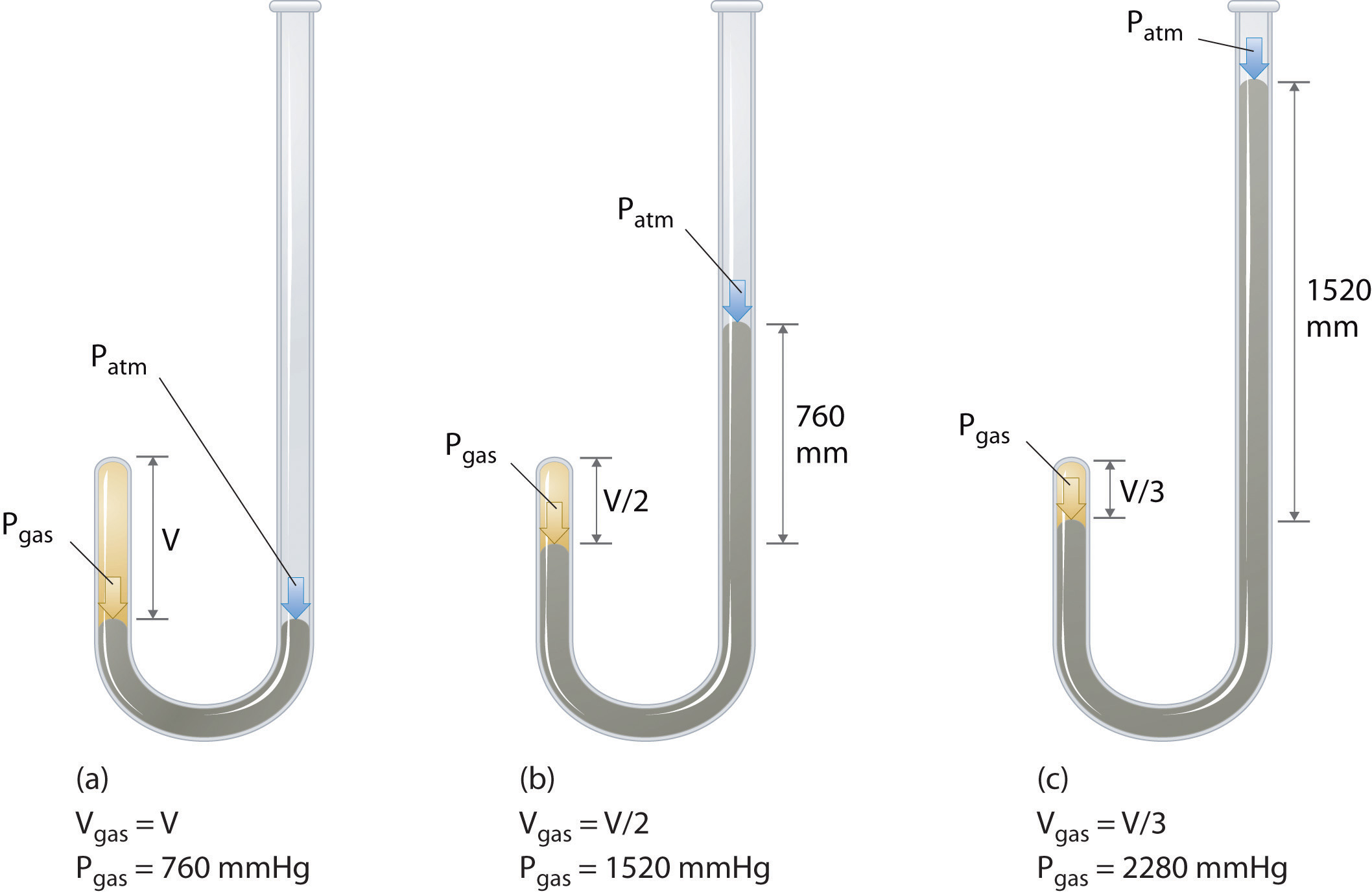
The Irish chemist Robert Boyle (1627–1691) carried out some of the earliest experiments that determined the quantitative relationship between the pressure and the volume of a gas. Boyle used a J-shaped tube partially filled with mercury, as shown in Figure \(\PageIndex{1}\). In these experiments, a small amount of a gas or air is trapped above the mercury column, and its volume is measured at atmospheric pressure and constant temperature. More mercury is then poured into the open arm to increase the pressure on the gas sample. The pressure on the gas is atmospheric pressure plus the difference in the heights of the mercury columns, and the resulting volume is measured. This process is repeated until either there is no more room in the open arm or the volume of the gas is too small to be measured accurately. Data such as those from one of Boyle’s own experiments may be plotted in several ways (Figure \(\PageIndex{2}\)). A simple plot of \(V\) versus \(P\) gives a curve called a hyperbola and reveals an inverse relationship between pressure and volume: as the pressure is doubled, the volume decreases by a factor of two. This relationship between the two quantities is described as follows:
\[PV = \rm constant \label{10.3.1} \]
Dividing both sides by \(P\) gives an equation illustrating the inverse relationship between \(P\) and \(V\):
\[V=\dfrac{\rm const.}{P} = {\rm const.}\left(\dfrac{1}{P}\right) \label{10.3.2} \]
or
\[V \propto \dfrac{1}{P} \label{10.3.3} \]
where the ∝ symbol is read “is proportional to.” A plot of V versus 1/P is thus a straight line whose slope is equal to the constant in Equations \(\ref{10.3.1}\) and \(\ref{10.3.3}\). Dividing both sides of Equation \(\ref{10.3.1}\) by V instead of P gives a similar relationship between P and 1/V. The numerical value of the constant depends on the amount of gas used in the experiment and on the temperature at which the experiments are carried out. This relationship between pressure and volume is known as Boyle’s law, after its discoverer, and can be stated as follows: At constant temperature, the volume of a fixed amount of a gas is inversely proportional to its pressure. This law in practice is shown in Figure \(\PageIndex{2}\).

At constant temperature, the volume of a fixed amount of a gas is inversely proportional to its pressure
The Relationship between Temperature and Volume: Charles's Law
Hot air rises, which is why hot-air balloons ascend through the atmosphere and why warm air collects near the ceiling and cooler air collects at ground level. Because of this behavior, heating registers are placed on or near the floor, and vents for air-conditioning are placed on or near the ceiling. The fundamental reason for this behavior is that gases expand when they are heated. Because the same amount of substance now occupies a greater volume, hot air is less dense than cold air. The substance with the lower density—in this case hot air—rises through the substance with the higher density, the cooler air.
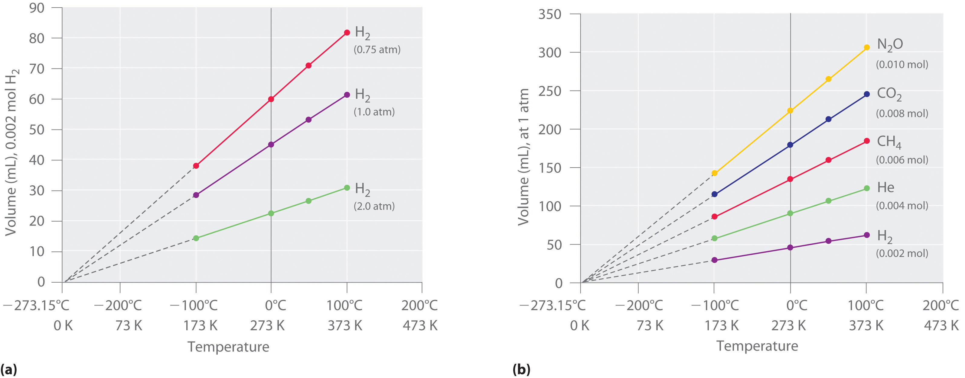
The first experiments to quantify the relationship between the temperature and the volume of a gas were carried out in 1783 by an avid balloonist, the French chemist Jacques Alexandre César Charles (1746–1823). Charles’s initial experiments showed that a plot of the volume of a given sample of gas versus temperature (in degrees Celsius) at constant pressure is a straight line. Similar but more precise studies were carried out by another balloon enthusiast, the Frenchman Joseph-Louis Gay-Lussac (1778–1850), who showed that a plot of V versus T was a straight line that could be extrapolated to a point at zero volume, a theoretical condition now known to correspond to −273.15°C (Figure \(\PageIndex{3}\)).A sample of gas cannot really have a volume of zero because any sample of matter must have some volume. Furthermore, at 1 atm pressure all gases liquefy at temperatures well above −273.15°C. Note from part (a) in Figure \(\PageIndex{3}\) that the slope of the plot of V versus T varies for the same gas at different pressures but that the intercept remains constant at −273.15°C. Similarly, as shown in part (b) in Figure \(\PageIndex{3}\), plots of V versus T for different amounts of varied gases are straight lines with different slopes but the same intercept on the T axis.

The significance of the invariant T intercept in plots of V versus T was recognized in 1848 by the British physicist William Thomson (1824–1907), later named Lord Kelvin. He postulated that −273.15°C was the lowest possible temperature that could theoretically be achieved, for which he coined the term absolute zero (0 K).
We can state Charles’s and Gay-Lussac’s findings in simple terms: At constant pressure, the volume of a fixed amount of gas is directly proportional to its absolute temperature (in kelvins). This relationship, illustrated in part (b) in Figure \(\PageIndex{3}\) is often referred to as Charles’s law and is stated mathematically as
\[V ={\rm const.}\; T \label{10.3.4} \]
or
\[V \propto T \label{10.3.5} \]
with temperature expressed in kelvins, not in degrees Celsius. Charles’s law is valid for virtually all gases at temperatures well above their boiling points.
The Relationship between Amount and Volume: Avogadro's Law
We can demonstrate the relationship between the volume and the amount of a gas by filling a balloon; as we add more gas, the balloon gets larger. The specific quantitative relationship was discovered by the Italian chemist Amedeo Avogadro, who recognized the importance of Gay-Lussac’s work on combining volumes of gases. In 1811, Avogadro postulated that, at the same temperature and pressure, equal volumes of gases contain the same number of gaseous particles (Figure \(\PageIndex{4}\)). This is the historic “Avogadro’s hypothesis.”

A logical corollary to Avogadro's hypothesis (sometimes called Avogadro’s law) describes the relationship between the volume and the amount of a gas: At constant temperature and pressure, the volume of a sample of gas is directly proportional to the number of moles of gas in the sample. Stated mathematically,
\[V ={\rm const.} \; (n) \label{10.3.6} \]
or
\[V \propto.n \text{@ constant T and P} \label{10.3.7} \]
This relationship is valid for most gases at relatively low pressures, but deviations from strict linearity are observed at elevated pressures.
For a sample of gas,
- V increases as P decreases (and vice versa)
- V increases as T increases (and vice versa)
- V increases as n increases (and vice versa)
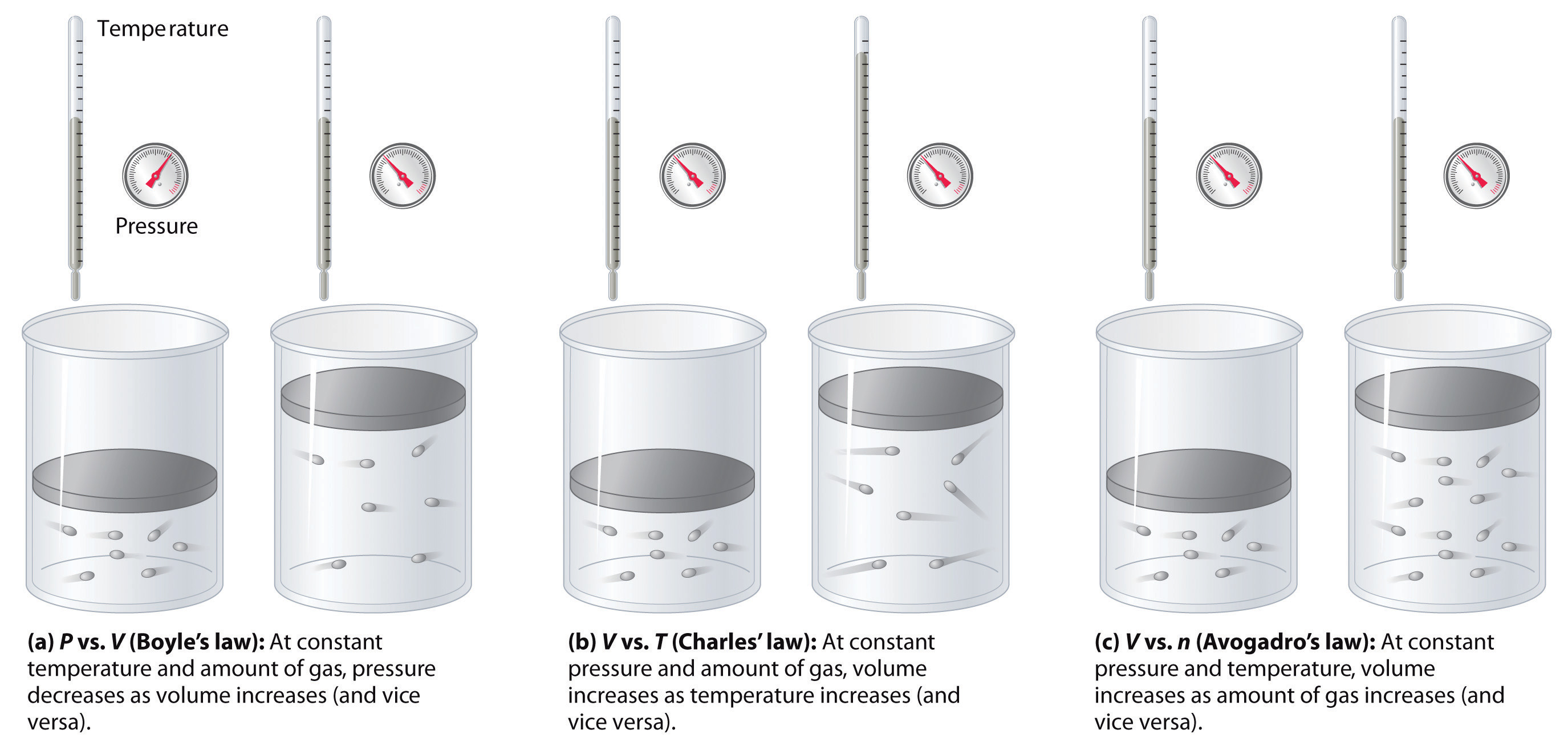
The relationships among the volume of a gas and its pressure, temperature, and amount are summarized in Figure \(\PageIndex{5}\). Volume increases with increasing temperature or amount, but decreases with increasing pressure.

Summary
The volume of a gas is inversely proportional to its pressure and directly proportional to its temperature and the amount of gas. Boyle showed that the volume of a sample of a gas is inversely proportional to its pressure (Boyle’s law), Charles and Gay-Lussac demonstrated that the volume of a gas is directly proportional to its temperature (in kelvins) at constant pressure (Charles’s law), and Avogadro postulated that the volume of a gas is directly proportional to the number of moles of gas present (Avogadro’s law). Plots of the volume of gases versus temperature extrapolate to zero volume at −273.15°C, which is absolute zero (0 K), the lowest temperature possible. Charles’s law implies that the volume of a gas is directly proportional to its absolute temperature.

